Eigenvalue analysis and Parallelization of the
Multi-grid
Preconditioned
Conjugate Gradient Method
Osamu
Tatebe* (建部修見)Department of Information Science, Facultyof Science, the Universityof Tokyo
7-3-1
Hongo, Bunkyo-ku, Tokyo 113,JAPAN
1
Introduction
The multi-grid preconditioned conjugate gradient method(MGCG method)[12] is the PCG
method with the multi-grid method[ll] as a preconditioner. The MGCG method has the
fol-lowing properties.
1. Even in thecase that the problem is stiff and ill-conditioned, the MGCG methodconverges
fast.
2. The number of iterations ofthe CG method is very few.
3. The number of iterations does not depend upon a grid size.
In order to explain this phenomenon, this paper considers eigenvalue analysis, which is closely related to the number ofCG iterations. Since the MGCG method has these characters, it is an ideal method which solves the Poisson’s equations, and no other method has these characters. Next parallelization of the MGCG method is considered.
In thesection 2, the model of problems is described. Inthesections 3 and4,thepreconditioned
conjugate gradient method and the multi-grid method which are the basis of the MGCG method
areexplained and thesection 5 presentstheMGCG method. In the section6, eigenvalueanalysis
is shownthat the multi-gridpreconditioner suits the conjugate gradient method. In thesection 7,
parallelization of the MGCG method is considered. Under this consideration, the section 8
presents implementation of the MGCG method on the Fujitsu multicomputer AP1000 and its evaluation.
2
The
model of problems
The target problem is two-dimensional elliptic partial differential equation and the numerical
experiment is performed for thefollowing Poisson’s equation with Dirichlet boundary conditions
$-\nabla(k\nabla u)=f$ in $\Omega\subset\Re^{2}$ with $u=f_{\Gamma}$ on $\Gamma$
where $k$ is a real function, $\Omega$ is a domain in the two-dimensional space, $\Gamma$ is its boundary. This
equation is discretized by the finite element method and the system oflinear equations $Ax=f$
is obtained. This coefficient matrix$A$ is sparse, symmetric and positive definite.
3
The
preconditioned
conjugate
gradient method
If a real $n\cross n$ matrix $A$ is symmetric and positive definite, the solution of the linear system
$Ax=f$ is equivalent to the minimization of the quadratic function
$Q(x)= \frac{1}{2}x^{T}Ax-f^{T}x$
.
(1)The conjugategradient method is one of the minimization method and use A-conjugate vectors
as the direction vectors which are generated sequentially. Theoretically this method has the
striking property that the number of steps until convergence is at most rank$(A)$ steps. And
this method can be adapted successfully to the parallel and vector computation, since one CG
iteration requires only oneproduct of the matrix and the vector, twoinnerproducts, tree linked
triads, two scalar divides and one scalar compare operation.
Next the preconditioned conjugate gradient method is explained. Let $U$ be a nonsingular
matrix, and define $\tilde{A}=UAU^{T}$, then solve $\tilde{A}\tilde{x}=\tilde{f}$ by the use of plain conjugate gradient
method. Let $x^{0}$ be an initial approximatevector,then an initial residual$r^{0}$ is$r^{0}=f-Ax^{0}$
.
Let$M=U^{T}U,\tilde{r}^{0}=Mr^{0}$ and an initial direction vector $p^{0}=\tilde{r}^{0}$
.
The PCG algorithm is describedby Program 1.
$i=0$;
while (! convergence) $\{$
$\alpha_{i}=(\tilde{r}_{i}, r_{i})/(p_{i}, Ap_{i})$;
$x_{i+1}=x_{i}+\alpha_{i}p_{i}$; $r_{i+1}=r_{i}-\alpha_{i}Ap_{i}$; convergencetest; $\tilde{r}_{i+1}=Mr_{i+1}$; $\beta_{i}=(\tilde{r}_{i+1},r_{i+1})/(\overline{r};, r;)$; $p_{i+1}=\tilde{r}_{i+1}+\beta_{i}p_{i}$; $i++$; $\}$
Program 1: the PCG iteration
In the loop block of Program 1, an matrix $M$ at $\tilde{r}_{i+1}=Mr_{i+1}$ is not actually calculated, and
in ordinary circumstances, such as incomplete Cholesky decomposition CG method, only $M^{-1}$ is
got. Hence thefollowing equation:
$M^{-1}\tilde{r}_{i+1}=r_{i+1}$ (2)
must be solved.
This paper focuses on a solver of this equation (2) and new proposal is the PCG method
4
The
multi-grid
method
In case of the iterative method, the residual reduces most rapidly on the grid corresponding to the frequency components of it. The multi-grid method make good use of this characteristic and exploit alot ofgrids to aim at the convergence as rapid as possible in point ofthe iterative method.
These grids are leveled and numbered from thecoarsest grid. The number is called level
num-$ber$. The basicelement of the multi-grid method is
defect
correctionprinciple, which theresidualis reduced moving it from grid to grid. Defect correction scheme consists of three processes:
finer
grid
coarser
grid
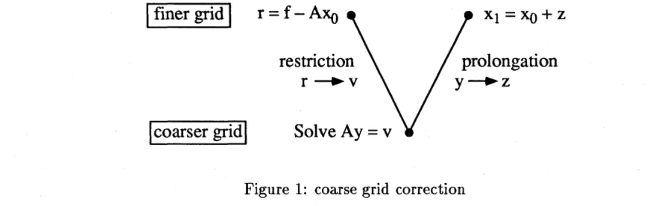
Figure 1: coarse grid correction
pre-smoothing process, coarse grid correction and post-smoothing process, and it uses only two
grids. In the pre-smoothing process the residual reduces by relaxant calculation on a finer grid.
In coarse grid correction(depicted in Fig. 1), theresidual$r$, which is not completely solvedin the
pre-smoothing process, is restricted tofit on a coarser grid, vector $v$, and the equation $Ay=v$
is solved on the coarser grid by the use of any method and the answer vector $y$ is prolonged on
the original finer grid, vector $z$, then the vector $x_{0}$ ofthe pre-smoothing process is corrected as
$x_{1}=x_{0}+z$
.
In post-smoothing process the residual also reduces by relaxant calculation on thefiner grid.
It is the two-grid method that this scheme is used only once per iteration and in the coarse
grid correction vector$y$ is solvedcorrectly enough. Besides, in thecoarse grid correction ifvector
$y$ is solved by the use ofrecursive call of the defect correction scheme, this method becomes the
multi-grid method.
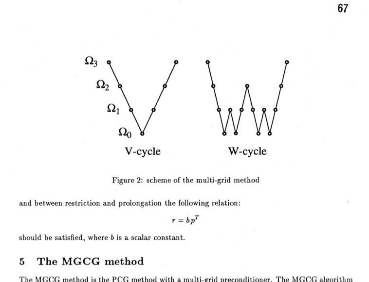
Many variations of how to call the defect correction procedure recursively is considerable.
Fig. 2 shows V-cycle scheme and W-cycle scheme. $\Omega_{i}$ means the grid oflevel number $i$. V-cycle
schemeis only one recursive call used in coarse grid correction and W-cycle scheme is two.
In the smoothing process, various methods, such as ILU, ADI and zebra relaxation, are
proposed. One purpose of this research is, however, formation of the efficient method with high
parallelism. Therefore iterative method with high parallelism, such as point Jacobi method and
multi-color SSOR method, is used as smoothing method.
A operation of transfera vectoron acoarser grid toavector on a finer grid callsprolongation,
andopposite operator calledrestriction. And the matrixpresentedthe operation of prolongation
is wrote $p$in this paper, and restriction $r$
.
In the following section, the equation of grid level $i$ is described as
V-cycle
W-cycle
Figure 2: scheme ofthe multi-grid method
and between restriction and prolongation the following relation:
$r=bp^{T}$
should be satisfied, where $b$ is a scalar constant.
5
The MGCG method
TheMGCG method is thePCG method with a multi-grid preconditioner. The MGCG algorithm
solving alinear equation $L_{l}x=f$is described as the Program 2. Let $x^{0}$ be an initial approximate
vector, then an initial residual $r^{0}$ is $r^{0}=f-L_{l}x^{0}$
.
Then $L_{l}\tilde{r}^{0}=r^{0}$ is relaxed by the multi-gridmethod, and an initial direction vector $p^{0}$ is equal to $\tilde{r}^{0}$
.
$i=0$; while (! convergence) $\{$ $\alpha_{i}=(\tilde{r}_{i},r_{i})/(p_{i}, L_{l}p_{i})$; $x_{i+1}=x_{i}+\alpha_{i}p_{i}$; $r_{i+1}=r;-\alpha_{i}L_{l}p_{i}$; convergence test;Relax $L_{l}\tilde{r}_{i+1}=r_{i+1}$ using the Multi-grid method
$\beta_{i}=(\overline{r}_{i+1}, r_{i+1})/(\tilde{r}_{i}, r_{i})$;
$p_{i+1}=\tilde{r}_{i+1}+\beta_{i}p_{i}$; $i++$;
$\}$
Program 2: the MGCG method
There are several variations of the multi-grid preconditioner. What method is used as the
multi-grid method? What method is used as a relaxant method? What cycle is used in the multi-grid
method? If $m$ is a cycle of the multi-grid method, $l$ is a relaxant method,
of iterations of the relaxant method and $g$ is the number of grids, MGCG method is shown
MGCG$(l, m,n,g)$
.
But $g$ is anoptional parameter. For example, MGCG$(RB, 1,2)$ is the MGCGmethod of the V-cyclemulti-grid preconditioner with two iterations ofRed-Black SSOR method as arelaxant calculation.
6
Eigenvalue
Analysis
In order to realize an efficiency ofa multi-grid preconditioner, the eigenvalues’ distribution of
a coefficient matrix after preconditioning is examined. The number of iterations of the
conju-gate gradient method until convergence depends upon an initial vector, the distribution of the
eigenvalues of a coefficient matrix and right-hand term. But in these factors the eigenvalues’
distribution is particularlyimportant.
Two-dimensional Poisson equation with Dirichlet boundary condition:
$-\nabla(k\nabla u)=f$ in $\Omega=[0,1]\cross[0,1]$
with $u=g$ on $\partial\Omega$
is considered. $k$ is a diffusion constant, $f$ is a source term and
$g$ is a boundary condition. The
experiment is performed in the following condition.
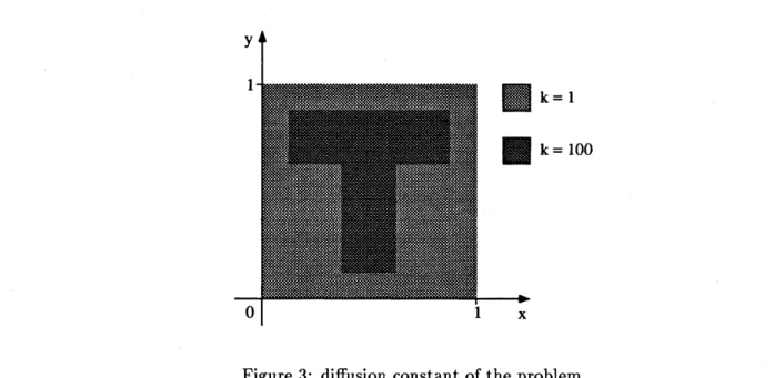
The diffusion constants $k$ is depicted by Fig. 3. This problem has the non-uniform diffusion
$k=1$
$k=100$
Figure 3: diffusion constant of the problem
constants and the shapeof the large diffusion constants is $T’$, therefore it has rich distribution
of the eigenvalues of the problem matrix. This problem is discretized to the mesh of 16 $\cross 16$
by the control volume method. The condition number of this coefficient matrix is 5282.6. The
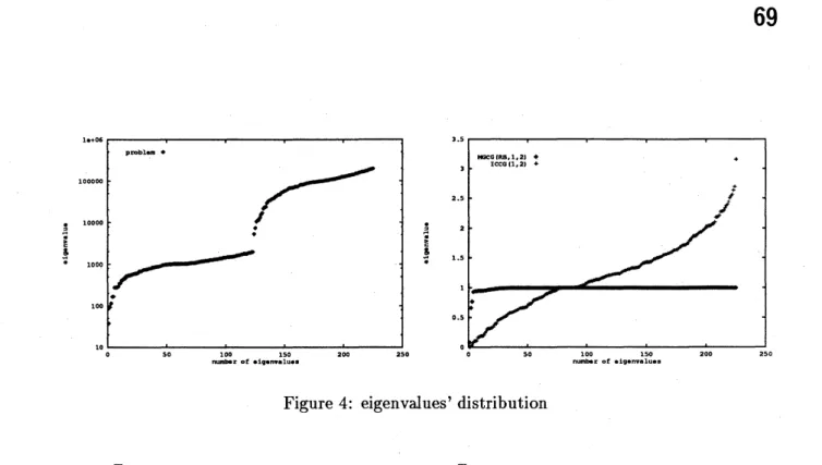
eigenvalues’ distribution of the problem matrix and the eigenvalues’ distribution of the matrix
after preconditioning is shown at Fig. 4. In order to compare, the preconditioning is occurred
both the multi-grid method and the incomplete Cholesky decomposition.
The matrix after the multi-grid preconditioning is calculated as follows. Let the matrix
Figure 4: eigenvalues’ distribution
as $M=U^{T}U$
.
Then eigenvalues of the matrix $UL_{l}U^{T}$ is investigated. On the other hand thematrix using the ICCG method is calculated as follows. The matrix $L_{l}$ is incomplete Cholesky
decomposed as $L_{l}=S^{T}S-T$, and the general eigenvalue problem $L_{l}x=\lambda S^{T}Sx$is solved.
The eigenvalues’ distribution of the multi-grid preconditioner is effective for the conjugate
gradient method as the following points:
1. eigenvalues are crowded almost around 1.
2. the least eigenvalue is increased.
3. the condition number is decreased.
These characteristicsare all desirable to the conjugate gradient method.
7
Parallelization
In this section, the parallelization of the MGCG method on a multicomputer is discussed. A
Multicomputer is a computer that has multiple processors and lacks a shared memory. All
communicationandsynchronization betweenprocessorsmusttake placethroughmessagepassing.
7.1
Parallelization
ofthe MGCG methodTheMGCG method is the PCG methodwith a multi-gridpreconditioner,so both the CG method
and themulti-grid method have to be parallelized. The CG method is easily parallelizedbut the
multi-grid method has the following problems.
1. The smoothing method must have high parallelism.
2. When the grid size is coarser, the overhead of communication is obvious.
3. When the grid size is coarser, the utilization of processors decreases. Idle processors appear
However the multi-grid method is very effective,ifthe following restrictions is satisfied.
1. A strong smoothing method that have poor parallelism is used in order to solve complex
and ill-conditioned problems.
2. The multi-grid method solves exactly on the finest grid in order to get fast convergence.
When the multi-grid method is parallelized, the former three problems are not settled and the
parallelization of the multi-grid method is severe. Therefore it has been invented the parallel
multi-grid method[3] not being equal to the stock serial multi-grid iJgorithm.
TheMGCG method,however,uses the multi-gridmethod as only a preconditioner of the PCG
method, so it is dispensable that the multi-grid method must use a strong smoothing method
and must exactly solveon the finest grid. In other words, these tworestrictions can beloosened
within the scope that a good performance of the target machine is gain. Of course, the looser
these restrictions are, the worse a speed of the convergence is. Therefore there is a trade-off
between the performance of the target machine, both communication and computation, and a speed of the convergence.
A smoothing method of the MGCG method should be a fineiterative method with high
par-allelism, therefore the Red-Black symmetric SOR method(RB-SSOR method) is selected. Then
thereis a trade-off between the number of grids used, a scheme of the multi-grid method and the
number ofiterationsof the RB-SSOR method, and the performance ofthe target machine.
7.2
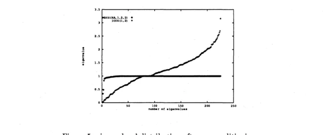
Eigenvalue analysisThis section considers a multi-grid preconditioner that utilizes fewer grids and does not exactly
solve on the finest grid. The problem is the same problem of the section 6, and the multi-grid
preconditioner uses only two-grid and on the coarsest grid the equationis not exactly solvedbut
relaxedbythesmoothing method. Theeigenvalues’distribution of the matrixafter
precondition-ing is shown at Fig. 5. In order to compare usual method, the preconditioning is occurred both
the multi-grid method and the incomplete Cholesky decomposition. The eigenvalues’
distribu-$\dot{arrow\iota g}\dot{r}$
Figure 5: eigenvalues’ distribution after preconditioning
samereason of the section 6 and in comparison with the incomplete Cholesky decomposition, the
multi-grid method is very effective preconditioner. Therefore as long as the multi-gridmethod is
used for a preconditioner, it is realized that the two restrictions of the section 7.1 do not haveto
be required for the MGCG method.
7.3
Domain Decomposition
This section presents the domain decomposition for the implementation of the MGCG method
on multicomputer. A product of the matrix and the vector, a restriction and a prolongation
of the multi-grid method, and a smoothing method require nearest-neighbor communications.
Therefore it is desired that data in one processor are allocated continuously if possible. If $M$
processors are connected by atorus network, thefollowing two methods are considerable.
(A) The domainofthedifferential equation is splitted into subdomains $M\cross 1$ which are assigned
to the processors of the system.
(B) The domain of the differential equation is splitted into subdomains $\sqrt{M}\cross\sqrt{M}$which are
assigned to the processors ofthe system.
Let problem size be $N$
.
The computation complexity and the communication complexity ofthese two methods are discussed. The computation complexity is proportional to the number of
inner grids, so the computation complexity of both methods is $0(N/M)$
.
The communicationcomplexity is proportional to the number of grids of subdomain’s edge, so the communication
complexityofthemethod (A) is $O(\sqrt{N})$ and the method (B) $O(\sqrt{N}/\sqrt{M})$
.
However the numberofcommunications of the method (B) is larger than it of the method (A). Therefore the larger
problemsize and processors are, the more profitable the method (B) is.
8
Implementation
on
the
APIOOO
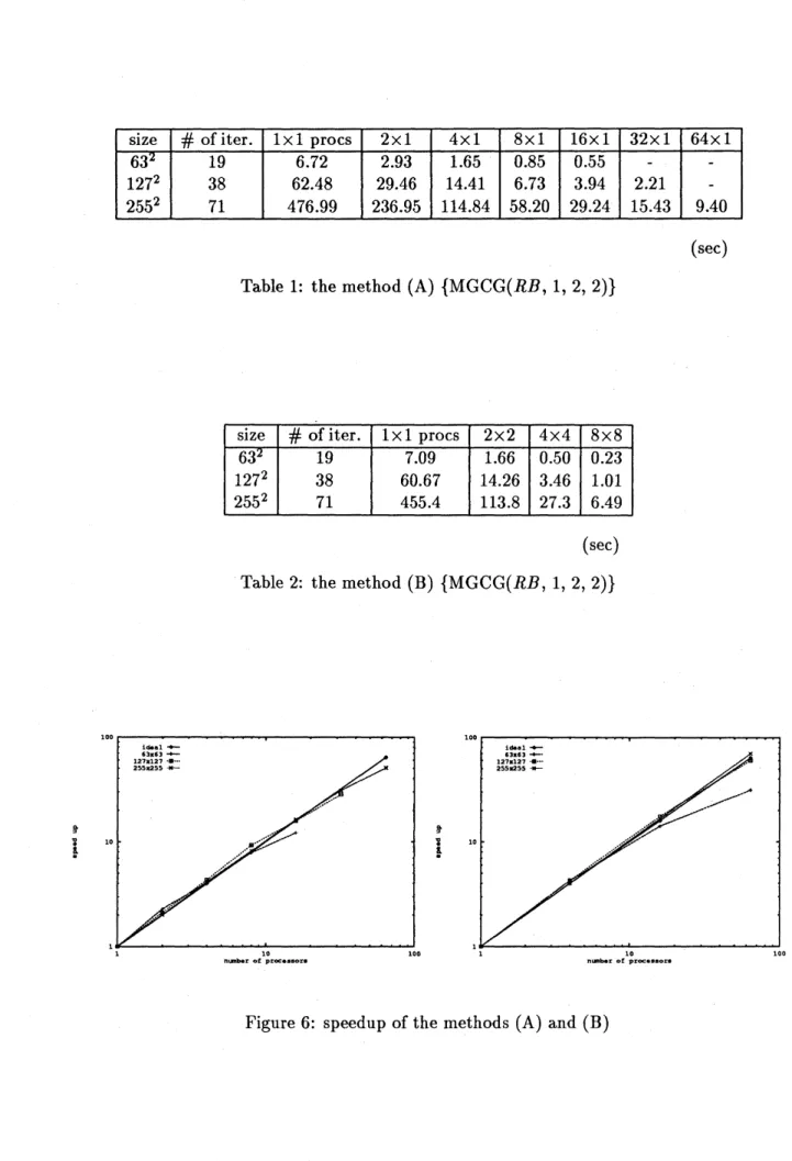
Two methods (A), (B) of the previous section is implemented on the Fujitsu multicomputer
AP1000. The numerical experiments is performed by MGCG(RB, 1, 2, 2) which exploits only
twogrids. The problem is two-dimensional Poisson equation with Dirichlet boundary condition:
$-\nabla(k\nabla u)=f$ in $\Omega=[0,1]\cross[0,1]$ with $u=g$ on $\partial\Omega$,
where$k$ is a constant. The problem is discretized tothe three kind of meshes: $64\cross 64,128\cross 128$
and 256 $\cross 256$, by the control volume method. The result is tables 1, 2 and a speedup of
these methods is shown at Fig. 6. These tables and figures indicate the method (B) is more
advantageous than the method (A) when a problem size is larger and the number of processors
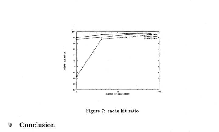
is larger. Both graphs are superlinear. This is because the problem size is fixed and the number
ofprocessors increases. Therefore the number ofdata in one processor decreases, and the cache
hit ratio and the hit ratio of line-send increase. Line-send is a special function of AP1000 and
datais directly transferredfrom a cache memory if this dataexists in the cache. Cache hit ratio
$(\sec)$
Table 1: the method (A)
{MGCG
$(RB,$ $1,2,2)$}
$(\sec)$
Table 2: the method (B)
{MGCG
$(RB,$ $1,2,2)$}
$3\sim$
$\sim.i$
$\frac{o}{\#,u}$
$\not\geq$
$l:*$
Figure 7: cache hit ratio
9
Conclusion
This paperfirstly considers eigenvalue analysis in orderto verify the effectof the MGCG method
which is a promising method as the solution of a large-scaled sparse, symmetric and positive
definitematrix. The eigenvalues’ distribution ofthe multi-grid preconditioner is effective for the
conjugate gradient method as the following points: 1. eigenvalues are crowded almost around 1. 2. the least eigenvalue is increased.
3. the condition number is decreased.
These characteristics are all desirable tothe conjugate gradient method. Secondly parallelization
of the MGCG method on multicomputerlacking a shared memory is discussed. The multi-grid
method has some problems when it is effectively parallelized, but the multi-grid preconditioner
of the CG method is sufficiently efficient even iftworestrictions of section 7.1 is not satisfied and
the performance of multicomputer is exploited.
References
[1] Adams, L. M., Iterative Algorithms
for
Large Sparse Linear System on Parallel Computers.PhD thesis, University ofVirginia, November 1982.
[2] Chan, T. F. andR. S.Tuminaro, “Analysisofa ParallelMultigrid Algorithm,” in Proceedings
of
thefourth
Copper MountainConference
on Multigrid Method(J. M.et al, ed.), pp. 66-86,Apri11989.
[3] Frederickson, P.
0.
and0.
A. McBryan, “Recent Developments for the PSMG MultiscaleMethod,” in Multigrid Methods III (W. Hackbusch and U. Trottenberg, eds.), vol. 98 of
[4] Hackbusch, W., “Convergence of Multi-Grid Iterations Applied to Difference Equations,”
Mathematics
of
Computation, vol. 34,no. 150, pp. 425-440, 1980.[5] Hackbusch, W., “Mult-grid ConvergenceTheory,” in Multigrid Methods(W. Hackbusch and
U. Trottenberg, eds.), vol. 960 of Lecture Notes in Mathematics, pp. 177-219,
Springer-Verlag, 1982.
[6] Hackbusch, W., “Multi-GridMethods and Applications”. Springer-Verlag, 1985.
[7] Maitre,J. F. and F. Musy, “Multigrid Methods: ConvergenceTheoryin a Variational
Frame-work,” SIAM J. Numer. Anal.,vol. 21, pp. 657-671, 1984.
[8] Moji, J. J., Parallel Algorithms and Matrix Computation’. Oxford University Press, 1988.
[9] Ortega, J. M., ”Introduction to Pamllel and Vector Solution
of
Linear Systems’. PlenumPress, 1988.
[10] Sbosny, H., “Domain Decomposition Method and Parallel Multigrid Algorithms,” in
Multi-gridMethods: Special Topics andApplications$\Pi$(W. Hackbuschand U. Trottenberg, eds.),
no. 189 in GMD-Studien, pp. 297-308, May 1991.
[11] St\"uben,K. and U. Trottenberg, “Multigrid Methods: FundamentalAlgorithms, Model
Prob-lem Analysis and Applications,” in Multigrid Methods(W. Hackbusch and U. Trottenberg,
eds.), vol. 960 of Lecture Notes in Mathematics, pp. 1-176, Springer-Verlag, 1982.
[12] Tatebe,
0.
and Y. Oyanagi, “The Multi-grid Preconditioned Conjugate Gradient Method,”in IPSJSIMNotes, 92-NA-42, pp. 9-16, August 1992. SWoPP’92.
[13] Wesseling, P., “Theoretical and practical aspects ofa muligridmethod,” SIAM Journal on