STOCHASTIC SEDIMENT DEPOSITION PROCESSES OF LARGE RESERVOIRS IN JAPAN

(1)

STOCHASTIC SEDIMENT DEPOSITION PROCESSES OF LARGE RESERVOIRS IN JAPAN

Tetsuya SUMI¹and Sameh A. KANTOUSH²

1. Water Resources Research Center, Disaster Prevention Research Institute, Kyoto University, Uji-shi, Japan, ([email protected])

2. Water Resources Research Center, Disaster Prevention Research Institute, Kyoto University, Uji-shi, Japan, ([email protected])

ABSTRACT

Sediment deposition and its accumulation as a function of time in years in a large reservoir depend on the flow and sediment hydrographs. In this paper, a stochastic sediment deposition in Japanese reservoirs is discussed. In Japan, sediment deposition in large reservoirs has been measured annually since the 1930. Such long-term annual sedimentation records are unique and represent some of the most useful global data to assess temporal trends in total sediment yields from larger catchments.

There are two objectives to use that small probability of the huge extreme event of sediment in:

predicting and design the operation and to propose new countermeasure. Among several probability distribution models, GEV (Generalized Extreme Value) model is the best goodness of fit to actual annual sedimentation records and each extreme sedimentation records has been evaluated by return period of 1/50-1/200 yrs.

1. INTRODUCTION

Sediment delivery to rivers is probably the most problematic off-site consequence of soil erosion in catchments. The input of sediment by erosion processes into rivers, reservoirs and ponds results in high sediment deposition rates and frequent dredging operations (Verstraeten and Poesen, 2001).

Predicts of temporal variation of sediment yield are needed for design of flood bypass system, and studies of reservoir sedimentations and river morphology. The evaluation of sediment yield in rivers, where total load consists predominantly of suspended load, plays an important role in the design of soil and water conservation and sediment control practices as well as in the design and management of dams, and other hydraulic structures. To this end, stochastic modelling techniques have been applied successfully to obtain reliable estimates of sediment yield. These techniques are superior to traditional methods which make use of discharge-concentration rating curves. Stochastic modelling accounts for the time series nature of rainfall, runoff and sediment yield processes (Anselmo et al., 1981; Sharma et al., 1979). It was used for short sampling intervals by Anselmo et al. (1981). An accurate estimate of sediment yield and reservoir sediment deposition rates should be made during the planning of new reservoirs. At present, sediment yield predictions are achieved mainly through simple empirical models that relate the annual sediment delivery by a river to catchment properties, including drainage area, topography, climate and vegetation characteristics (e.g. Verstraeten and Poesen, 2001). The amount of sediment trapped in a reservoir during a certain period of time is the difference between the sediment carried into the reservoir by the inflow and the sediment released with the outflow. Several deterministic methods have been developed to predict the amount of sediment carried into a reservoir as a function of watershed characteristics (Ackermann and Corinth, 1962; Gupta, 1974).

Reservoir sediments typically represent an important record of a catchment's erosion history.

Reservoir based studies have been successfully applied as a means of reconstructing long-term sediment yields (e.g. Labadz et al., 1991). However, most have limited temporal resolution and are unable to generate information on seasonal or event-scale processes. The complexity of catchment sediment delivery and reservoir sedimentation mechanisms means that most physically-based or mechanistic models are highly parameterized and require extensive field calibration.

(2)

Japanese watersheds are frequently affected by very heavy storms with daily precipitation of more than 300 mm, which causes significant sediment erosion. In Japan, sediment deposition behind certain large dams has been measured annually since the 1930’s (Miyazaki and Onishi, 1996;

Hiramatsu et al., 2002). Such long-term annual sedimentation records are unique and represent some of the most useful global data to assess temporal trends in total sediment yields from larger catchments. Miyazaki and Onishi (1996) examined the timing of sediment supply and transport by comparing annual rainfall data with changes in the volume of dam deposits. Imaizumi and Sidle (2005) investigated the relationship between sediment supply and transport processes in Miyagawa dam catchment. In Miyagawa Dam 11 catchment, percentages of landslides reaching channels varied from 56% in 1997–2000, 12 to 75% in 1976-1981, and were correlated with the maximum hourly rainfall.

In civil engineering practice many parameter estimation methods for probability distribution functions are in circulation. The choice of statistical estimation methods for probability distribution functions is one of the most challenging problems within civil engineering, and one that is filled with many controversies. Many attempts (for instance, Burcharth and Liu, (1994), and Van Gelder and Vrijling, (1997)), have been made to find out which estimation method is preferable for the parameter estimation of a particular probability distribution in order to obtain a reliable estimate of the p-quantiles.

In Fill and Stedinger (1995), it was shown that for realistic generalized extreme value (GEV) distributions and short records, a simple index-flood quantile estimator performs better than two- parameter (2P) GEV quantile estimators with probability weighted moment (PWM) estimation using a regional shape parameter and at-site mean and L-coefficient of variation (L-CV), and full three- parameter at site GEV/PWM quantile estimators. However, as regional heterogeneity or record lengths increase, the 2P-estimator quickly dominates. Fill and Stedinger (1995) generalizes the index flood procedure by employing regression with physiographic information to refine a normalized T-year flood estimator. In Naghavi and Yu (1996), it is shown that the quantile prediction accuracy of the log- Pearson type III (LP3) distribution depends largely on the accuracy of the parameter-estimation method used. In Takara and Stedinger (1994) the use of two-parameter distributions is recommended from the viewpoint of quantile estimation accuracy for datasets having sample skewness greater than 0.38 and less than 1.8. They found that the quantile lower bound estimators are likely to provide more accurate quantile estimators than other procedures.

Extreme-regime sedimentation is commonly of interest in lake sediment research because of its associations with hydrologic and geomorphologic catchment hazards (e.g., Gomez et al. 2002). The emphasis of such studies is usually on temporal variability in the sedimentary record. Comparatively little research has been carried out on the within-reservoir areal variability of sedimentation (e.g., Gilbert, 2003).

In this paper, a stochastic sediment deposition in Japanese reservoirs is discussed. There are two objectives to use that small probability of the huge event of sediment in: predicting and design the operation and to propose new countermeasure. Based on annual sedimentation records in Japanese reservoirs, several probability distribution models are compared by the goodness of fit from the viewpoint of quantile estimation accuracy and each extreme sedimentation records has been evaluated by the selected model.

2. RESERVOIR SEDIMENTASTION IN JAPAN

In Japan, approximately 2,730 dams over 15 meters in height have been constructed for water resource development or flood control purposes, but the total reservoir storage capacity is only up to 23 billion m3. The sediment yields of the Japanese rivers are relatively high due to the topographical, geological and hydrological conditions and this has consequently caused sedimentation problems to those reservoirs.

Based on the annual research conducted for 877 reservoir which have gross storage capacities of over one million m3, specific sediment yields in these catchment areas are ranging from several hundred to several thousand m3/km2/year, and the specific sedimentation volume becomes higher in central high mountainous regions along the Median Tectonic Line and the Itoigawa-Shizuoka Tectonic Line as shown in Figure 1.

(3)

単位は㎥/㎢/年

m³/km²/yr

Figure 1 Specific reservoir sedimentation volume in Japan

Annual storage capacity losses in those reservoirs are ranging approximately from 1.0 to 0.1 %. In other words, it is noted that the reservoir lives are approximately 100 to 1000 years. Reservoir sedimentation problems are represented by such as the siltation of intake facilities, aggradations of upstream river bed, reservoir storage capacity loss and, sometimes, lack of sufficient sediment supply to downstream which may cause river bed degradation or coastal erosion.

3. STOCHASTIC SEDIMENT DEPOSITION IN RESERVOIRS 3.1 Annual Sedimentation records in Reservoirs

Figure 2 shows Tenryu river system which is one of the highest sediment yield rates in Japan. In the middle reach, Sakuma dam was constructed in 1957 by J- Power. Figure 3 shows annual sedimentation record in Sakuma dam. After completion, high rates up to 4.3 million m3/yr had been recorded for 1957-1969. After that, it has been gradually decreased such as to 1.65 and 1.55 million m3/yr for 1970-1982 and 1983-2001, respectively. This is because that slope protection works in the upstream catchments have been progressed and, also, extreme flood events caused by large typhoons have not been fitted in these years.

Figure 4 shows annual sedimentation record in Miwa and Koshibu dams which are located upstream of the Tenryu river as shown in Figure 3. These were constructed by the Ministry of Land, Infrastructure, Transport and Tourism (MLIT) for multipurpose dams.

In the Tenryu river, there was a large flood in 1982 caused by severe rainy front which produced extreme sedimentation in these reservoirs at the same time. In Miwa and Koshibu reservoirs, they were more than 15 times and 6 times of the average annual ones and

Sakuma dam Miwa dam

Koshibu dam

Sakuma dam Miwa dam

Koshibu dam

(4)

Sakuma Dam

-10,000 0 10,000 20,000 30,000 40,000 50,000 60,000 70,000 80,000 90,000 100,000 110,000 120,000 130,000

1956 1957 1958 1959 1960 1961 1962 1963 1964 1965 1966 1967 1968 1969 1970 1971 1972 1973 1974 1975 1976 1977 1978 1979 1980 1981 1982 1983 1984 1985 1986 1987 1988 1989 1990 1991 1992 1993 1994 1995 1996 1997 1998 1999 2000 2001 2002 2003 2004 2005 2006 -1,000 0 1,000 2,000 3,000 4,000 5,000 6,000 7,000 8,000 9,000 10,000 11,000 12,000 13,000

Yaers

Annual sedimentation(1,000ｍ3) Sedimentation（1,000ｍ³）

Planned sedimentation capacity

Planned sedimentation Annual sedimentation

Actual sedimentation

Average annual sedimentation

Figure 3 Annual sedimentation records in Sakuma dam Miwa Dam

-2,000 0 2,000 4,000 6,000 8,000 10,000 12,000 14,000

1956 1957 1958 1959 1960 1961 1962 1963 1964 1965 1966 1967 1968 1969 1970 1971 1972 1973 1974 1975 1976 1977 1978 1979 1980 1981 1982 1983 1984 1985 1986 1987 1988 1989 1990 1991 1992 1993 1994 1995 1996 1997 1998 1999 2000 2001 2002 2003 2004 2005 2006 -1,000 0 1,000 2,000 3,000 4,000 5,000 6,000 7,000

Yaers

Actual sedimentation

Average annual sedimentation

Koshibu Dam

-4,000 0 4,000 8,000 12,000 16,000 20,000 24,000

1956 1957 1958 1959 1960 1961 1962 1963 1964 1965 1966 1967 1968 1969 1970 1971 1972 1973 1974 1975 1976 1977 1978 1979 1980 1981 1982 1983 1984 1985 1986 1987 1988 1989 1990 1991 1992 1993 1994 1995 1996 1997 1998 1999 2000 2001 2002 2003 2004 2005 2006 -500 0 500 1,000 1,500 2,000 2,500 3,000

Yaers

Average annual sedimentation Actual sedimentation

Figure 4 Annual sedimentation records in Miwa and Koshibu reservoirs

(5)

Yahagi Dam

-2,000 0 2,000 4,000 6,000 8,000 10,000 12,000 14,000 16,000

1956 1957 1958 1959 1960 1961 1962 1963 1964 1965 1966 1967 1968 1969 1970 1971 1972 1973 1974 1975 1976 1977 1978 1979 1980 1981 1982 1983 1984 1985 1986 1987 1988 1989 1990 1991 1992 1993 1994 1995 1996 1997 1998 1999 2000 2001 2002 2003 2004 2005 2006 -750 0 750 1,500 2,250 3,000 3,750 4,500 5,250 6,000

Yaers

Average annual sedimentation Actual sedimentation

Figure 5 Annual sedimentation records in Yahagi reservoirs

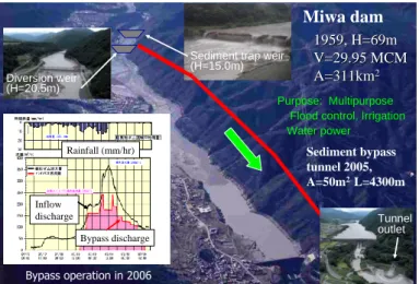
1959, H=69m 1959, H=69m V=

V=29.95 MCM29.95 MCM A=311kmA=311km²²

Sediment bypass tunnel 2005, A=50m²L=4300m Purpose: Multipurpose

Flood control, Irrigation Water power

Miwa dam

Bypass discharge Inflow

discharge

Rainfall (mm/hr)

Bypass operation in 2006

Sediment trap weir (H=15.0m) Diversion weir

(H=20.5m)

Tunnel outlet

Figure 6 Sediment bypass scheme at Miwa dam, Tenryu River

These extreme events have been also occurred in other dams such as at Yahagi dam as shown in Figure 5. In 2000, a severe flood disaster caused by rainy front had also yielded huge amount of sediment from the catchments and extreme sedimentation was produced after that.

In case of Miwa dam completed in 1959, extreme runoff events occurred in 1959, 1961, 1982 and 1983 causing serious disasters and sediment yield in the river basin. Since 1966, gravel have been constantly removed according to a maintenance plan and then approximately 5.32 million m3 sediment have been dredged in 33 years up to 1998. If those gravel is not removed, the total sedimentation is approximately 19.47 million m3, and estimated the mean annual sedimentation is 0.47 million m³. From the view point of the eternal reservoir sedimentation management, a sediment bypass system (comprised of a 20.5m high diversion weir and a 4,300m long bypass tunnel with a maximum discharging capacity of 300m³/s) is constructed in March 2004 to reduce sedimentation of the reservoir. Figure 6 shows the schematic diagram of the bypass system. During large flood event in 2006, almost half of flood flow containing high sediment concentration was diverted through bypass tunnel (Red line).

In Koshibu dam and Yahagi dam, almost the same sediment bypass systems are under construction.

In case of designing these structures, we should consider the stochastic characteristics of flood events

(6)

3.2 Stochastic Analysis of Annual Sedimentation Records 3.2.1 Frequency Analysis of Hydrological Extreme Events

Based on the annual sedimentation records, we can evaluate probability of these extreme events.

Takara, K. (2009) shows frequency analysis of hydrological extreme events as follows.

We have been regarding hydrological events as random variables. Frequency of hydrological extreme events is therefore a concern of decision makers in practical works for water resources planning and hydraulic design of flood control facilities. To describe the probability distribution of a random variable X, we use a cumulative distribution function. The value of this function Fx (

x

) is simply the probability P of the event that the random variable takes on value equal to or less than the argument:

Fx (

x

)=P [X

 x

] (1) This is the probability that during the year the random variable in question, X, will not exceed some

x

; Fx (

x

) is, therefore, regarded as non-exceedance probability. Hereafter, we use a simpler expression F (

x

) for Fx (

x

). The probability density function

f ( x )

of X is related to F (

x

) as:

F (

x

) =



 x

dt t

f ( )

(2)

For a particular value or threshold

x

_p with a non-exceedance probability p, there is a relationship:

T =

) 1 (

1 p

n 

(3)

in which T is the return period or recurrence interval (year) that corresponds to the hydrological variable X = x_p and n is the annual average number of occurrence of X during the period in which F(

x

) is estimated. x_p is often called as quantile or T -year event. Note that if we deal with annual maximum data series, n = 1:

T =

1  p

1

(4)

The 50-year event (T = 50) has a non-exceedance probability p = 0.98. Likewise, T = 100 then p = 0.99 and T = 200 then p = 0.995. Since p = F (x_p), if we set T or p, we can obtain the quantile (T -year event) x_p by using the inverse function of F :

x

_p= F^-1(p) (5) which gives the value of x_p corresponding to any particular value of p or T. Now the frequency of hydrological extreme value (annual maximum value) is related to frequency, return period or non- exceedance probability.

3.2.2 Probability Distribution Models

There are many reasonable probability distributions (frequency analysis models) for modeling extreme events. Important families include the normal, extreme-value type I and type II, and Pearson type III (or Gamma) distributions.

(7)

The probability density function (pdf) of the lognormal distribution with three parameters (LN3) is:

 





 





 



 

  

 



2

) ln(

2 exp 1 2 ) ( ) 1 (

Y

c

Y

x c

x x

f 







⁽⁶⁾

in which

x

is a hydrological variable; a is lower bound parameter;



_Y= the mean of y = ln (x - a);



_Y= the standard deviation of y. Its cumulative distribution function (CDF) is in a from of the well-known standard normal distribution function



as:

 

^s ^t ^dt

x y

F ^s

Y

Y 



 











 



 







2

2 exp 1 2 ) 1

(

 



(7)

in which

Y

y

Y

s 



 

is the reduced (or standardized) variable of the original variable y. The Gumbel

distribution's CDF is:

 

 



 



 



  



 a

c x x

F ( ) exp exp

(8)

The generalized extreme-value (GEV) distribution has a CDF with a parameter k



0:

 





 



 



 



  





k

a c k x x

F

1

1 exp )

(

(9)

If k = 0, the GEV distribution is equivalent to the Gumbel distribution shown as Eq. (8). Another family Pearson type III (Gamma) distribution's CDF for c<

x

<



is:

( ) , x c / ( a ) G

x

F   

 



 

  

(10)

where

 (a )

is the gamma function and G (a, x) is the "incomplete gamma function" defined as:

^ ^ 

0^ ^ ^

1

,

)

(  e

^u

u

^

du ^G ^x ^ 

0^x

^e

^^u

^u

^

^du

)

1

,

( 

^ (11) For a set of hydrologic extreme-value time series data (annual maxima data), hydrologists often try several distributions and select one to calculate the estimate of quantile (T-year event) x_p for a concerned non-exceedance probability p, which corresponds to the return period T by using Eq. (5).

Note that we can obtain analytical solutions for the extreme-value theory such as the Gumbel and GEV distributions, respectively:

 p  c

a

x

_p

  ln  ln 

(12)

and

 ^p  ^c

k

x

_p

  a (  ln )

^k

 1 

(13)

(8)

However, since the families of the normal and Pearson type III distributions cannot have such analytical solutions, they require computational solutions. Many statistical textbooks include the standard normal distribution table, which shows the computational solutions for this purpose.

If we had sufficient knowledge of a hydrologic phenomenon, one could derive its population probability distribution without depending on observed data. If we had sufficiently long record of the phenomenon, we could determine its frequency distribution precisely, as long as the distribution did not change over time. But we should select a model that approximates the population distribution based on the limited knowledge and data generally available. When fitting distributions to a set of hydrologic extreme-value time series data, we often find that several distributions achieve almost the same goodness of fit, but can generate different estimates of extreme quantiles.

Takara and Takasao (1990) propose an attractive model selection procedure. Conventional model selection procedures have generally used goodness-of-fit criteria and/or tests. When two or more distributions achieve almost the same good results in fitting, the proposed procedure will select the final distribution in terms of both the goodness of fit and the stability of quantile estimators, which is preferable from a practical viewpoint. While it is not difficult to estimate quantile variability, quantile accuracy (which is really of greater concern) is more difficult to determine because the true distribution of the events and its associated parameters are unknown. Takara and Stedinger (1994) summarized Monte Carlo studies comparing and evaluating various fitting methods for the lognormal (LN), Pearson type III (PHI), log-Pearson type III (LPIII), Gumbel (EV1) and generalized extreme-value (GEV) distributions. To screen candidate distributions, Takara and Takasao (1990) used Standard Least Squares Criterion (SLSC) to evaluate goodness of fit of each distribution to a hydrological extreme- value dataset quantitatively.

3.2.3 Return Period of Annual Sedimentations in Reservoirs

Based on the procedure proposed by Takara and Takasao (1990), we selected suitable probability distribution models for annual sedimentation records in Miwa, Koshibu and Yahagi dams which are shown in Figures 4 and 5. Table 1 shows selected models and calculated annual sedimentation volumes for several return periods. Generalized extreme-value (GEV) distribution is the best fitting in three dams. Based on the model, we can estimate return periods of actual maximum annual sedimentation such as from 1/58 yrs to 1/170 yrs. We should consider the small probability of these huge events in both operating and assessing long term sustainability of reservoirs. It is also important to optimize designing of countermeasures such as capacity of sediment bypass tunnels.

Table 1 Return Period of Annual Sedimentation in Miwa, Koshibu Yahagi dams

Data number 50 Data number 38 Data number 31

Function Gev Function Gev Function Gev

SLSC 0.063 SLSC 0.042 SLSC 0.057

1/2 years 125 1/2 years 248 1/2 years 184

1/20 years 1,372 1/20 years 1,404 1/20 years 1,193

Volume Return period Volume Return period Volume Return period 4,241 1/105 years 2,404 1/58 years 2,830 1/170 years

SLSC: Standard Least Squares Criterion (Takara and Takasao, 1990) Gev: Generalized Extreme-Value Distribution Model

Unit: 1,000m³

Actual maximum annual sedimentation

(1,000ｍ³)

Actual maximum annual sedimentation

(1,000ｍ³) Actual maximum

annual sedimentation (1,000ｍ³)

Miwa Dam Koshibu Dam Yahagi Dam

(9)

4. CONCLUSIONS

Sediment deposition and its accumulation as a function of time in years in a large reservoir depend on the flow and sediment hydrographs. In this paper, a stochastic sediment deposition in Japanese reservoirs is discussed as follows.

1) In Japan, sediment deposition in large reservoirs has been measured annually since the 1930.

Such long-term annual sedimentation records are unique and represent some of the most useful global data to assess temporal trends in total sediment yields from larger catchments.

2) During more than 30 yrs operation, we can find several extreme annual sedimentations mostly caused by severe rainfall events. In order to evaluate these extreme sedimentation volumes, probability distribution models can be used as the same as other hydrological extreme events.

3) Based on annual sedimentation records in Japan, several distribution models have been compared by the goodness of fit from the viewpoint of quantile estimation accuracy which procedure is proposed by Takara and Takasao (1990).

4) Generalized extreme-value (GEV) distribution is the best fitting probability distribution model in Miwa, Koshibu and Yahagi dams. Based on the model, we can estimate return periods of actual maximum annual sedimentation in these dams such as from 1/58 yrs to 1/170 yrs.

5) We should consider the small probability of these huge events from the view point of return period and sedimentation volume in one event, both in operating reservoir for long term sustainability and in optimized designing of countermeasures such as capacity of sediment bypass tunnels.

5. REFERENCES

Ackermann, C.W. and Corinth, R.L. (1962). An empirical equation for reservoir sedimentation. Int.

Assoc. Sci. Hydrol. (I.A.S.H.), 59: 359--366.

Anselmo, V., Galmacci, G., Singh, V.P. and Ubertini, L. (1981). Rainfall-runoff-sediment yield modelling by stochastic models: preliminary results. Annali Facolt Agraria, Universit di Perugia, Italy XXXV.

Burcharth, H.F., and Liu, Z. (1994). On the extreme wave height analysis. In Port and Harbour Research Institute, Ministry of Transport, editor, International Conference on Hydro-Technical Engineering for Port and Harbour Construction (Hydro-Port), Yokosuka, Japan, pages 123-142, Yokosuka: Coastal Development Institute of Technology.

Fill, H.D., and Stedinger, J.R. (1995). Homogeneity tests based upon Gumbel distribution and a critical appraisal of Dalrymple’s test, Journal of Hydrology. v 166 p 81-105.

Fill, H.D., and Stedinger, J.R. (1998). Using regional regression within index flood procedures and an empirical Bayesian estimator. Journal-of-Hydrology. SEP 1998; 210 (1-4): 128-145.

Gilbert R. (2003). Spatially irregular sedimentation in a small, morphologically complex lake:

implications for paleoenvironmental studies. J. Paleolimnol. 29: 209–220.

Gomez B., Page M., Bak P. and Trustrum N. (2002). Self-organized criticality in layered, lacustrine sediments formed by landsliding. Geology 30: 519–522.

Gupta, S.K., (1974). A distributed digital model for estimation of flows and sediment load from large ungaged watershed. Ph.D. Thesis. University of Waterloo, Waterloo, Ont., 354 pp.

Hiramatsu, S., Kuroiwa, T., and Arasuna, T. (2002). Influence of changes of deforestation area and reforestation area on sediment yield. Journal of the Japan Society of Erosion Control Engineering, 55(4), 3–11.

Imaizumi, F. and Sidle, R. C. (2005). Relationship between sediment supply and transport process in

(10)

Labadz, J. C, Burt, T. P. and Potter, A. W. R. (1991). Sediment yield and delivery in the blanket peat moorlands of the southern penniness, Earth surf. Processes and landforms 16, 255-271.

Miyazaki, Y., and Onishi, S. (1996). Study on the relation between the sediment and the rainfall.

JSCE, 533, 41–50.

Naghavi, B., and Yu, F. X. (1996). Selection of parameter-estimation method for LP3 distribution.

Journal-of-Irrigation-and-Drainage-Engineering. v 122 n 1 Jan-Feb 1996, p 24-30.

Rendon-Herrero, O., Singh, V. P. and Chen, V. J. (1980). ER-ES Watershed relationship. Proc. Int.

Symp. on Water Resources Systems (Roorkee, India), vol. I, 11-8-41 to 11-8-47.

Sharma, T. C., Hines, W. G. S. and Dickinson, W. T. (1979) Input-output model for runoff-sediment yield processes. J. Hydrol. 40, pp. 299-322.

Singh, V. P. and Chen, V. J. Singh, V. P. (1982). On the relation between sediment yield and runoff volume. Modelling Components of the Hydrologic Cycle pp. 555-570. Water Resources Publications, Littleton, Colorado, USA

Takara, K. and Stedinger, J.R. (1994). Recent Japanese Contributions to Frequency Analysis and Quantile Lower Bound Estimators. Stochastic and Statistical Methods in Hydrology and Environmental Engineering, Vol. 1, pp. 217-234.

Takara, K. and Takasao, T. (1990). Evaluation of hydrologic frequency analysis models based on quantile variability obtained by resampling methods. Proc. Fifth International Conference on Urban Storm Drainage, Suita, Osaka, Japan, 2, pp. 587-592.

Takara, K. (2009). Frequency analysis of hydrological extreme events and how to consider climate change. Water Resources and Water Related Disasters under Climate Change, -Prediction, Impact Assessment and Adaptation-, 19th UNESCO-IHP Training Course, Kyoto University.

Verstraeten, G., Poesen, J. (2001). Factors controlling sediment yield from small intensively cultivated catchments in a temperate humid climate. Geomorphology 40, 123–144.

Van Gelder, P.H.A.J.M., and Vrijling, J.K. (1997). A comparative study of different parameter estimation methods for statistical distribution functions in civil engineering applications. Structural Safety and Reliability, Vol. 1, pp.665-668.