Crete Island, Greece, 5–10 June 2016
SHAPE IDENTIFICATION ANALYSIS OF CAVITY
IN RESIN STRUCTURE BASED ON THERMAL NONDESTRUCTIVE TESTING METHOD
K. Maruoka1, T. Kurahashi2, and T. Iyama3
1 Graduate School of Nagaoka University of Technology 1603-1 Kamitomioka, Nagaoka, Niigata, Japan
e-mail: [email protected]
2 Nagaoka University of technology 1603-1 Kamitomioka, Nagaoka, Niigata, Japan
e-mail: [email protected]
3 Nagaoka National College of Technology 888 Nishikatakai, Nagaoka, Niigata, Japan
e-mail: [email protected]
Keywords: Shape identification analysis, Thermal nondestructive testing method, Finite ele- ment method, Adjoint variable method, Gaussian filter.
Abstract. The shape identification analysis is carried out to obtain the unknown defects shape in the structure based on the finite element and the adjoint variable methods. In this study, the test piece including the known defect shape is employed to solve the shape identifi- cation problem. In addition, we present the shape identification problem of cavity in resin test piece made by 3D printer using the observed temperature on the test piece surface. It is known that the temperature on top of the test piece is not uniformly distributed, if there are cavities in the test piece. Furthermore, according to practical experiment, it has been con- firmed that the characteristic of the temperature distribution depends on cavities size. The thermal physical constants, i.e., the thermal conductivity and the convection coefficient, are identified for the model of the test piece including a cavity based on the experimental data, and the shape identification analysis is carried out. In the numerical analysis, the finite ele- ment method is applied to simulate the temperature distribution in the test piece, and the ad- joint variable method is employed to identify the cavity shape.
to find out defects, depending on the size and depth of the defects. On the other hand, by ap- plying a thermal testing method, studies to identify the defect shape by inverse analysis meth- od from time history of temperature [1, 2] is carried out. In previous studies, it is concluded that the corrosion shape of the concrete can be identified if assuming the initial corrosion shape as appropriate. In the fields of optimal control problems, the study about reduction of convergence for performance function [3, 4].
In this study, we use the resin structure created by 3D printer such that the shape of cavity is freely changed. The purpose of this study is to identify the cavity shape based on the in- verse analysis, and to carry out the improvement of the treatment in computation of the shape identification.
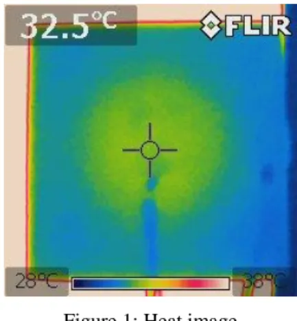
Figure 1: Heat image
2 EXPERIMENT BY THERMAL NONDESTRUCTIVE TESTING METHOD 2.1 Measurement situation
The photo of experiment is shown in Figure 2, and the drawing of test piece used this study is shown in Figure 3 (a). The sample has been made of ABS resin and created by 3D printer.
Then a test piece with a cavity having a thickness of 10mm and a test piece without cavity are also created. Pair of test pieces (15mm thickness cavity, no cavity) are set on hot plate, heated up for 1200 seconds, and thermal observation at two observation points on the surface with a thermocouple is carried out every 10 seconds. Observation point is placed on the upper sur- face of the thick point (Point A) and thin portion (Point B) of the cavity thickness (See Figure 3(b)).
2.2 Observational result
The measured temperature history at Point A and Point B is shown in Figure 4 (a) and (b).
As a result, without relation to presence or absence of the cavity, there are no big difference in temperature history observed at Point B. However, in Point A, it is confirmed a tendency that
Figure 2: Photo of observation
(a) Drawing of the test piece (b) Observation point Figure 3: Detail of the test piece
the temperature of the test piece with a cavity increases more than the test piece without a cavity at the same time. This is considered to effect due to the influence of heat transfer from the air which is heated in the cavity. Similar experiment are also carried out using a test piece with a cavity having a thickness of 10mm. The temperature history measured at Point A and Point B is shown in Figure 5 (a) and (b). From the results, it is found that the temperature dif- ference at Point A is small compared the case with a test piece cavity thickness 15mm. Thus, the thickness of the cavity difference, it can be seen that the result is a difference in the tem- perature history at the test piece surface.
3 SHAPE IDENTIFICATION ANALYSIS
Using thermal properties found out previous chapter, the shape identification analysis is carried out. Initial shape model is given as including the cavity thickness 13mm, we set target shape as cavity thickness 15mm.
3.1 State equation
Formulation in the shape identification analysis is described below. In this study, the whole domain of the test piece is denoted as Ω. Then temperature distribution satisfies heat transfer
(a)At Point A (b) At Point B Figure 4: Time history of temperature of resin surface (1)
(a)At Point A (b) At Point B Figure 5: Time history of temperature of resin surface (2)
equation shown in Equation (1). For the heat transfer equation, initial condition and boundary condition are defined as Equations (2).
0 c,ii
(1)
3 2
,
2 inf
1 ,
1 0
) (
) (
ˆ ) ˆ(
on h
n
on h
n on
in t
cav i
i i i
(2)
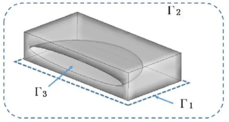
where ρ, c, κ, ni, h1, h2, infand cavdenote density, specific heat, thermal conductivity, unit normal vector, heat transfer coefficient of inside cavity, heat transfer coefficient of outside surface, surrounding temperature, temperature inside cavity. Γ1 means lower surface, Γ2
means outside surfaces, and Γ3 means surface of cavity (See Figure 6).
3.2 Performance function
To evaluate computed temperature history, following performance function is defined.
dt d R
J 21
tt0f
(obs)2 (3)
Figure 6: Boundary definition of the test piece
where tf, R, andobs mean heating termination time (Total time), weight diagonal matrix, ob- served temperature.
3.3 Lagrangian function
Applying adjoint variable λ, following Lagrangian function is obtained to minimize perfor- mance function [6, 7]. The adjoint variable method is one of the minimization technique of the performance function, and is suitable for the inverse problems such that a lot of unknown parameters should be solved.
dt d J
J*
tt0f
(c,ii) (4) First variation which is necessary condition that Lagrangian function become minimization is shown in equation (5). Stationary condition is given as condition that each terms equal zero.i i
x x J J
J
J J
* * * *
*
(5)
where xi indicates transplantable nodes.
3.4 Finite element equation
Shape function for four-node tetrahedral element is introduced into state equation to discre- tize the state equation spatially with Galerkin method. In addition, the equation is discretized in time based the Crank-Nicolson method. The finite element equation is shown in equation (6).
e e
e e
e} [H ]{ }{T} in
]{
c[Me
(6)
In equation (6), [Me], [He], and {Te} indicate:
dMe] e{ e}{ e}T
[ (7)
dHe] e{ ei}{ ei}T
[ , , (8)
ds q
ds q
Te}
{e}
{e}{ 2 3 (9)
where q means thermal flow late. Superposing finite element equation for individual domain, such equation can be represented as equation (10).
3 2 1
0 0 0
0 ) (
on S
on S
on in tf
(12)
3.6 Gradient vector of the Lagrangian function
Final term in equation (5) can be calculated with adjoint variable as following equation:
e t T
t i
in C dt
x
f
i i
i
*
} x x { } B x { } A J {
0 (13)
Nodal positions are updated with gradient vector. In this method, the update of the coordinate on cavity surface and the re-evaluation of the temperature difference at observation points are iteratively carried out according to steepest descent method [7].
3.7 Computational condition
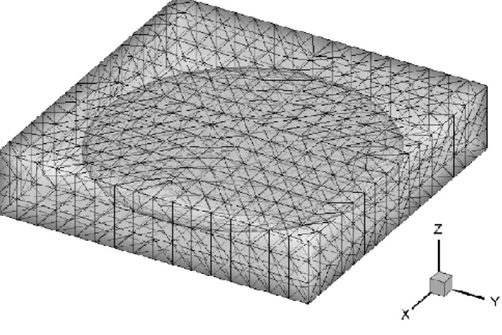
The finite element model of the test piece is shown in Figure 7. The model is composed four-node tetrahedral element. Total number of nodes are 1460, and total number of elements are 5552. The computational conditions are referred to experiment and given as Table 1. Thermal properties for the test piece is given as shown in Table 2 considering the thing which the ABS resin is not filled enough as shown in Figure 8. The observational data at Point A in the previous experiment (See Figure 4 (a)) is employed as observed temperature. In addition, the time history of temperature on the hot plate and temperature within the cavity as boundary conditions are shown in Figure 9 (a) and (b).
Figure 7: Finite element model
Total number of nodes Total number of elements Total time tf, sec
Time increment Δt, sec Time step
Convergence criterion ε
1460 5552 600 10 60 10-6
Table 1: Computational condition.
Density ρ Kg/m3
Specific heat c
J/(kg℃)
Thermal conductivity κ W/(m2℃)
Heat transfer coefficient h Outside surface
W/(m2℃)
Cavity W/(m2℃)
ABS 750 1386 0.1354 10.0 7.0
Table 2: Example of the construction of one table.
Figure 8: Cross-section of test piece
(a) On the hot plate (b) In the cavity Figure 9: Time history of temperature of resin surface
3.8 Computational result
Figure 10 (a) shows identified shape of the cavity and Figure 10 (b) shows variation of normalized performance function per iteration number. Final iteration number is 18, performance function is about 0.55 when converting initial performance function into 1. However surface of the cavity becomes un- dulation, targeted shape as 15mm thickness cavity cannot be obtained.
(a) The shape of the cavity at the final iteration (b) Variation of performance function Figure 10: Computational results (1)
4 SMOOTHING PROCESS
The smoothing process for gradient vector is introduced to modify the oscillation of the gradient vector with respect to coordinate on cavity surface. For the smoothing method, Gaussian filter [8] is employed. Looking at the surface of the cavity as two-dimensional sur- face, the gradient vector is smoothed.
4.1 Gaussian filter
Gaussian filter is a kind of the smoothing filter for the field of graphics. In smoothing method with Gaussian filter input of weighting parameter, value of the target nodes is determined by value of all nodes on the same plane. And the Gaussian filter has the advantage that the extent of the smoothing process is adjustable with the parameter σ. The weighting parameter in Gaussian filter [9] is defined as following equation:
2 2 2
2
2 2
y) 1
G(x,
y x
e
(14)
where x and y is the distance of x-axial distance and y-axial distance between the target node and referenced node. The weighting parameter becomes large value if the distance is short.
The parameter σ which is comparable to the variance in Gaussian distribution determines flat- tening of the distribution. In addition, as the summation of the weighting parameter for the target node becomes 1, we multiply the weighting parameter by the summation. The weighting parameter for node m to node n is shown in following equation:
cx
n
y y x x
y y x x
n m n m
n m n m
e e
1
2
) ( ) ( 2
2
) ( ) ( n) 2
(m,
2
2 ) ( ) ( 2 ) ( ) (
2
2 ) ( ) ( 2 ) ( ) (
2 1 2
1 G
(15) where cx means the number of nodes on the surface, x(m) and y(m) mean x-coordinate and y- coordinate of the node m. Then smoothed gradient vector is computed, the calculating formula is represented as following matrix form:
) (
* ) 2 (
* ) 1 (
*
) , ( )
2 , ( ) 1 , (
) , 2 ( )
2 , 2 ( ) 1 , 2 (
) , 1 ( )
2 , 1 ( ) 1 , 1 (
) (
* ) 2 (
* ) 1 (
*
cx cx
cx cx
cx
cx cx
cx x
J x
J x
J
G G
G
G G
G
G G
G
x J x
J x
J
(16)
4.2 Shape identification introducing Gaussian filter
In the Gaussian filter, the parameter σ is given as 20, and the shape identification analysis is carried out. The identified shape of the cavity is shown in Figure 11 (a). The surface of the cavity is smoother than the result without smoothing process in previous section. As the variation of performance func- tion, in the case using Gaussian filter, number of iteration is larger and performance function is lower (See Figure 11(b)). It is confirmed that the temperature comes closer to observed value by applying smoothing process.
(a) The shape of the cavity at the final iteration (b) Variation of performance function Figure 11: Computational results (2)
5 CONCLUSIONS
In this study, the shape identification problem of the cavity in the structure based thermal testing method is carried out. The test piece including a cavity that the shape is variable made by 3D printer is heated from undersurface and the temperature is observed. The shape identification analysis, based the finite element method for four-node tetrahedral element and adjoint variable method, discretizing equations spatially and temporally with Galerkin method and Crank-Nicolson method, is carried out. In the identification process, Gaussian filter is employed to smooth the movement of nodes. The results in this study are shown below.
When the test piece is heated from lower surface, the temperature of the test piece includ- ing a cavity is higher than the one without cavity at the same observation point and time, the temperature at face just above the cavity is especially high.
The temperature history of the test piece on heating changes depending on the cavity size, the temperature becomes highly as the cavity is larger.
Based on Observed Temperature on Concrete Surface, International Journal of Com- puter Science, 4:4:340-351, 2010.
[2] T.Kurahashi, H.Oshita, Shape Determination of 3-D Reinforcement corrosion in Con- crete Based on Observed Temperature on Concrete Surface, Computers and Concrete, 7:1:63-81, 2010.
[3] Z. Wang, I.M. Navon, X. Zou, F.X. Le Dimet, The second order adjoint analysis: theory and applications, Meteo. and Atmo. Phys. 50:3-20, 1992.
[4] Z. Wang, I.M. Navon, X. Zou, F.X. Le Dimet, A truncated Newton optimization algo- rithm in meteorology applications with analytic Hessian/vector products., Computation- al Optimization and Applications, 4:241-262, 1995.
[5] T. Kurahashi, M. Kawahara, Examinations for thermal condition of Lagrange multiplier for heat transfer control problems, International Journal for Numerical Methods in En- gineering, 73:982-1009, 2008.
[6] T. Kurahashi, Examination for adjoint boundary conditions in initial water elevation es- timation problems, International Journal for Numerical Methods in Fluids, 63:1270- 1295, 2010.
[7] Y. Sakawa, Y. Shindo, On global convergence of an algorithm for optimal control, IEEE Transactions on Automatic Control, 25:1149-1153, 1980.
[8] S. Wang, W. Li, Y. Wang, Y. Jiang, S. Jiang, R. Zhao, An improved Difference of Gaussian Filter in Face Recognition, Journal of Micromechanics and Microengineering, 7.6.429-433, 2012.
[9] H. Ishiwata, H. Kubota, Y. Shima, Experimental study on Gaussian filter in restoration of error diffused character images, Information Processing Society of Japan, 18, 5, 2006.