GEOLOGICAL, GEOPHYSICAL AND GEOCHEMICAL STUDIES ON THE HYDROTHERMAL SYSTEM OF MENENGAI
GEOTHERMAL FIELD, KENYA
イサク, キプロノ, カンダ
http://hdl.handle.net/2324/2236184
出版情報:九州大学, 2018, 博士(工学), 課程博士 バージョン:
権利関係:
GEOLOGICAL, GEOPHYSICAL AND GEOCHEMICAL STUDIES ON THE HYDROTHERMAL SYSTEM OF
MENENGAI GEOTHERMAL FIELD, KENYA
by
Isaack Kiprono Kanda
A Dissertation Submitted in Partial Fulfilment of the Requirement for the Degree of
Doctor of Engineering (Earth Resources Engineering)
Supervised by
Professor Dr. Yasuhiro Fujimitsu
Laboratory of Geothermics
Department of Earth Resources Engineering Graduate School of Engineering
Kyushu University – Japan
January, 2019
TABLE OF CONTENTS
LIST OF FIGURES ... i
LIST OF TABLES ... viii
ACKNOWLEDGMENTS ... ix
DEDICATION... xi
ABSTRACT ... xii
GENERAL INTRODUCTION ... 1-1 1.1. Background of the study ... 1-1 1.2. Geothermal status in Kenya ... 1-3 1.3. Previous studies ... 1-4 1.4. Purpose and plan of study ... 1-6 1.5. Structure of the dissertation... 1-8 References ... 1-10
FIELD CHARACTERISTICS OF MENENGAI GEOTHERMAL AREA ... 2-1 2.1. Introduction ... 2-1 2.2. Geology and structural setting... 2-1 2.2.1. Regional setting ... 2-1 2.2.2. Local geology... 2-3 2.2.3. Lineament studies ... 2-7 2.3. Hydrological setting ... 2-10 2.3.1. Regional Relief and Rainfall Distribution ... 2-10 2.3.2. Regional hydrology ... 2-12 2.3.3. Hydrological models ... 2-13 2.4. Conclusion ... 2-17 References ... 2-18 GRAVITY DATA ANALYSIS AND INTERPRETATION ... 3-1 3.1 Introduction ... 3-1
3.2 Gravity method: theory and application ... 3-1 3.3 Gravity survey ... 3-3 3.4 Gravity data reduction and Bouguer density estimation ... 3-4 3.4.1 Gravity data correction ... 3-4 a). Latitude correction (normal gravity) ... 3-5 b). Free-air correction ... 3-5 c). Bouguer correction ... 3-6 d). Terrain correction ... 3-6 3.4.2 Bouguer density estimation ... 3-8 a). Simple G-H method ... 3-8 b). F-H method ... 3-8 c). Extended F-H ... 3-9 d). Akaike's Bayesian Information Criterion (ABIC) ... 3-10 e). Comparison with the Variance of the Upward-Continuation (CVUR) ... 3-11 3.5 3-D gravity inversion ... 3-12 3.6 Results and Discussion ... 3-16 3.6.1 Bouguer density estimation ... 3-16 3.6.2 Bouguer anomaly ... 3-21 3.6.3 3-D gravity modeling... 3-23 3.7 Conclusion ... 3-32 References ... 3-33
RESISTIVITY STUDIES USING MAGNETOTELLURIC METHOD ... 4-1 4.1. Introduction ... 4-1 4.2. The magnetotelluric method... 4-1 4.3. Magnetotelluric in geothermal exploration ... 4-4 4.4. Magnetotelluric data acquisition, processing and analysis ... 4-8 4.4.1. Data acquisition ... 4-8 4.4.2. Distortion and static shift in MT methods ... 4-9 4.4.3. Dimensionality analysis ... 4-12 a). Swift-skew and ellipticity ... 4-13 b). Phase tensor ... 4-15 4.5. 1-D and 2-D Occam’s inversion of MT data... 4-19 4.6. 3-D ModEM inversion of MT data ... 4-20 4.7. Results and Discussion ... 4-22 4.7.1. MT inversion results ... 4-24 4.8. Conclusion ... 4-31
References ... 4-32
ISOTOPE AND WATER CHEMISTRY STUDIES ... 5-36 5.1. Introduction ... 5-36 5.1.1. Isotope geochemistry ... 5-36 5.1.2. Reactive transport modeling ... 5-38 5.2. Geochemistry in geothermal exploration ... 5-40 5.3. Physical and chemical characteristics of Menengai geothermal field... 5-40 5.4. Results and discussion ... 5-43 5.4.1. Major chemical elements studies ... 5-44 5.4.2. Isotope Studies ... 5-49 5.5. Reactive geochemical modeling... 5-53 5.5.1. Physical and chemical characteristics of MW-01 ... 5-53 5.5.2. Mineral and geochemical data ... 5-55 5.5.3. Equilibrium and kinetic considerations ... 5-61 5.5.4. Model setup ... 5-64 5.5.5. Results and discussion ... 5-66 5.6. Conclusion ... 5-73 References ... 5-74
COMBINED INTERPRETATION AND DISCUSSION ... 6-85 3.8 Introduction ... 6-85 3.9 Menengai caldera ... 6-85 3.10 The Olrongai area ... 6-93 3.11 Conclusion ... 6-99 References ... 6-100
GENERAL CONCLUSIONS ... 7-1 7.1. Introduction ... 7-1 7.2. Field characteristics ... 7-1 7.3. Gravity data analysis and interpretation ... 7-2 7.4. Resistivities studies using the MT method ... 7-3 7.5. Isotope and water chemistry studies... 7-3 7.6. Combined interpretation and discussion ... 7-4
i | P a g e
LIST OF FIGURES
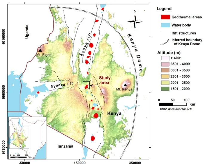
Figure 1.1: Map of Kenya showing the location of geothermal sites (in red) and the rift structures (black lines). Also indicated are water bodies (shown in light blue polygons) and major cities. ... 1-2 Figure 1.2: Schematic diagram that shows the stages and targets of the present studies. The
properties of wells are represented by x, P, T, h and M which represents chemical composition, Pressure, Temperature, enthalpy, and mass flow, respectively. ... 1-8 Figure 2.1: Location map of the study area. The high altitude (>1500 m above sea level) area shows
part of the Kenya dome. ... 2-3 Figure 2.2: Descriptive map of the study area showing the elevation (m), faults, fracture and
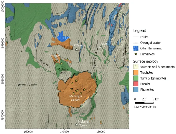
location of fumaroles. ... 2-5 Figure 2.3: Surface geology map of the study area, modified from previous work done by McCall
(1967), Jennings (1971) and Walsh (1969). ... 2-6 Figure 2.4: Lineament density map of the study area per km2. The Rose diagrams show the
azimuths direction of the local distribution of lineaments, with radial coordinate indicating the number of lineament. ... 2-9 Figure 2.5: Annual average rainfall and relief map of Kenya. ... 2-11 Figure 2.6: Main geological structures and local hydrology. The study area is shown in grey, and
the green line is considered as an area of interest from a hydrological perspective.
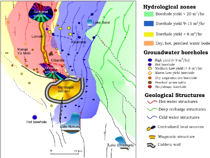
Major faults, perennial rivers and ephemeral rivers are indicated as broken red lines, blue lines and broken blue lines, respectively. ... 2-12 Figure 2.7: Hydrogeological controls of the Menengai geothermal area (adapted from Mungania
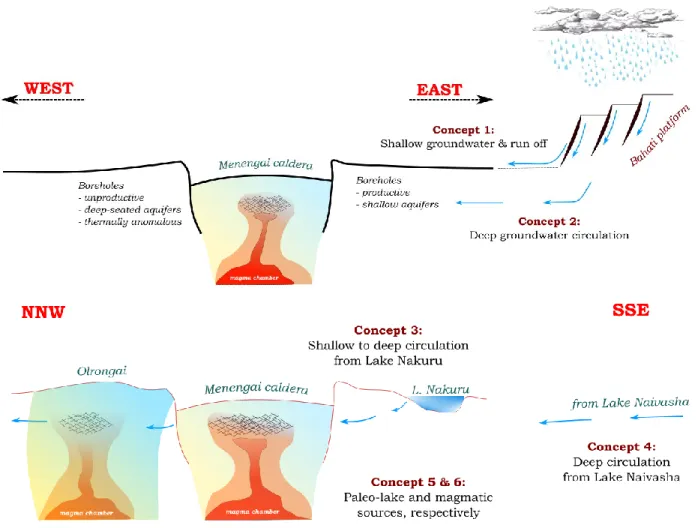
& Lagat, 2004). Boreholes are represented by circles. ... 2-14 Figure 2.8: Hydrogeological model of the study area indicating possible fluid recharge sources of
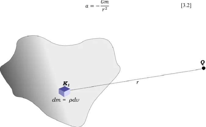
the geothermal system. ... 2-16 Figure 3.1: Geometry representation of the points 𝐾 and 𝑄 and distance 𝑟 between them; notations
of equation [3.3].. ... 3-2
ii | P a g e Figure 3.2: Reference model from the gridded density contrast of the down hole density estimated
from the initial 10 geothermal wells drilled in Menengai. ... 3-14 Figure 3.3: A 3-D Gravity inversion grid. The cell size is 620 m × 650 m × 50 m with the height
component set to increase by a factor of 1.08 for each successively deeper layer. The colored map represents complete Bouguer anomaly (CBA) with values ranging from - 189.4 mGal to -134.7 mGal. ... 3-15 Figure 3.4: Bouguer density by G-H method... 3-18 Figure 3.5: Bouguer density by the Simple F-H method ... 3-19 Figure 3.6: (a) Bouguer density by Extended F-H method, (b) Extended F-H density frequency
distribution. ... 3-20 Figure 3.7: The Bouguer density by Comparison with Variance of the Upward-Continuation
(CVUR). ... 3-21 Figure 3.8: Bouguer anomaly map calculated for a Bouguer density of 2.23 × 10³ kg m−3. ... 3-23 Figure 3.9: A planar view of density distribution at 1000 m asl elevation. ... 3-25 Figure 3.10: A planar view of density distribution at sea level. ... 3-26 Figure 3.11: A planar view of density distribution at 1000 m b.s.l elevation. ... 3-27 Figure 3.12: A planar profile and isosurface (2.45 × 10³ kg m−3) inferred from the density model
of Menengai area. ... 3-28 Figure 3.13: A display of geological faults as seen from the surface and fumaroles location
superimposed against a deep planar layer at sea level and an isosurface of 2.45 × 10³ kg m−3 to highlight the dense body of Olrongai hill. ... 3-29 Figure 3.14: A display of geological faults/caldera rim ring-fracture as seen from the surface and
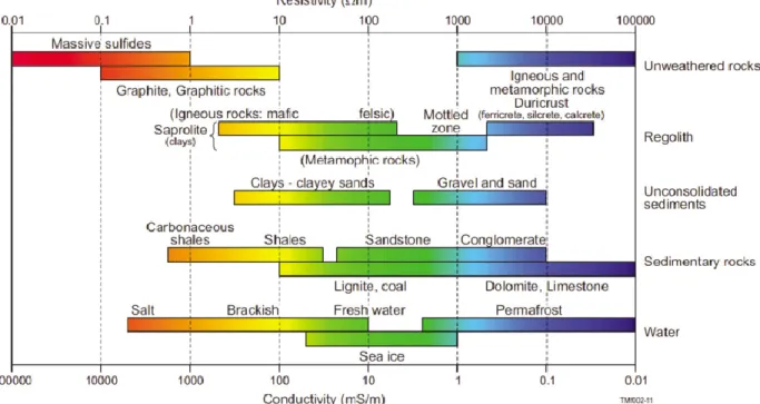
fumaroles location superimposed against a deep planar layer at sea level and an isosurface of 2.45 × 10³ kg m−3 to highlight the dense body of Menengai caldera. The inferred faults are presented as broken lines. ... 3-30 Figure 4.1: Resistivity and conductivity values of various rock-forming materials (from González- Álvarez et al., 2014; adapted from Palacky, 1988). ... 4-6 Figure 4.2: A conceptual model of a generic geothermal system with a 250 to 300°C geothermal
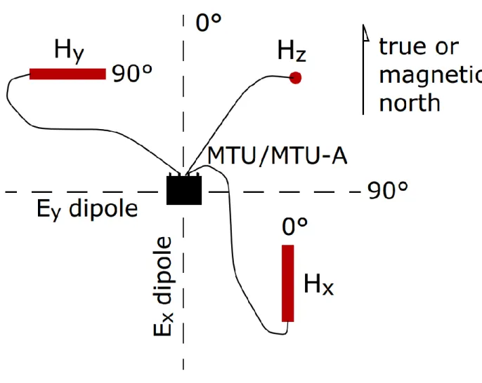
reservoir with isotherms, alteration zones, and structures. ... 4-7 Figure 4.3: Schematic representation of the field set-up for a typical 5-channel MT sounding
(adapted from Phoenix Geophysics Ltd., 2010). Ex and Ey dipoles represent the non-
iii | P a g e polarizing electrodes for measuring the electric field components. The magnetic induction coils indicated by Hx and Hy measure the horizontal components of the magnetic field, and Hz shows its vertical component. The directions are labeled as x, y, and z, whereas the E and H are the electric field and the magnetic field, respectively.
Hence, the acquisition unit records the time-series data of all five electromagnetic field components (i.e., Ex, Ey, Hx, Hy, and Hz). ... 4-8 Figure 4.4. Typical magnetotelluric data collected in the study area displayed as apparent
resistivity and phase curves. The curves on the left side show the raw data collected while those on the right side display the results after the removal of static shift and distortion. Period acts as a proxy for depth, with short periods sensing shallow structures and long periods sensing deeper structures. ... 4-11 Figure 4.5: Plots of all MT sounding curves of TE and TM modes from the 212 stations in
Menengai field. The red dots indicate the TE mode and the blue dots indicate TM mode.
The consistent shape of all the curves is displayed. ... 4-12 Figure 4.6: Swift-skew and ellipticity are plotted for selected MT stations. ... 4-14 Figure 4.7: Graphical representation of the phase tensor as an ellipse. The magnitudes of the
minimum and maximum principal axes are given by Φmin and Φmax, respectively.
If the phase tensor is non-symmetric, a third coordinate invariant is required to describe the tensor, which is the skew angle, β. The angle α – β gives the orientation of the major axis of the ellipse and defines the link between the tensor and the observational reference frame (x1 and x2); adapted from Caldwell et al. (2004). ... 4-16 Figure 4.8: Phase tensor maps for periods of (a) 0.0033 s, (b) 0.01 s, (c) 1 s, (d) 10 s, (e) 100 s, and
(f) 300 s. ... 4-18 Figure 4.9: Example of data misfit between observed and modeled station responses of the Zxy (red
dots) and Zyx (blue) components for some selected stations. The dots and the lines represent the measured values and modeled response, respectively. ... 4-23 Figure 4.10: Menengai caldera map showing 3-D MT inversion profiles (in blue) along E-W
directions (P1-P4) and S-N direction (P5-P8), and 2-D MT inversion profiles (in red) P9-P12. Four MT stations selected for 1-D Occam’s inversion are encircled in green.
The orientation of 2-D profiles was chosen to ensure it crosses near as much data as
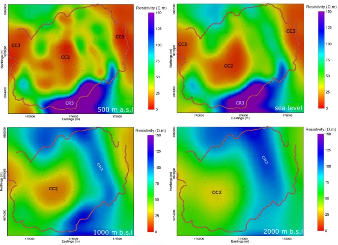
iv | P a g e possible. The black and orange dots show the MT stations and the caldera rim, respectively. ... 4-24 Figure 4.11: MT profiles along W-E directions (P1-P4). ... 4-25 Figure 4.12: MT profiles along S-N directions (P5-P8). ... 4-26 Figure 4.13: Horizontal slices at different heights above sea level through the 3-D resistivity model
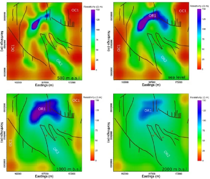
derived from inversion of the caldera MT dataset. The black and orange dots show the MT stations and the caldera rim, respectively. ... 4-27 Figure 4.14: Horizontal slices at different heights above sea level through the 3-D resistivity model
derived from inversion of Olrongai area MT dataset. The orange dots and brown lines denote fumaroles and faults, respectively. ... 4-28 Figure 4.15: 2-D resistivity models for profiles P9, P10, P11 and P12 of Menengai caldera as
shown in Figure 4.10. ... 4-29 Figure 4.16: 1-D resistivity models of the caldera area from MT stations 052, 006, 007 and 164
align from north to south (see Figure 4.10), respectively, and situated right above the low resistive body (CC2). ... 4-30 Figure 5.1: Governing equations for a single phase coupled reactive transport system (Steefel et
al., 2005). ... 5-38 Figure 5.2: Cl-SO4-HCO3 ternary diagram (after Giggenbach, 1988) showing the distribution of
major anions in the geothermal fluid of Menengai wells. The water type is predominantly bicarbonate (HCO3-). Various colored symbols are used to distinguish different wells. ... 5-41 Figure 5.3: Scatter plots of SiO2 versus CO2 (mg/kg) of Menengai well discharge waters collected
during the testing period. Similarly colored symbols represent different samples from the same well while the orange lines indicate hypothetical mixing boundaries. .... 5-45 Figure 5.4: Scatter plots of Na versus SiO2 (mg/kg) of Menengai well discharge waters collected
during the testing period. Similarly colored symbols represent different samples from the same well while the orange lines indicate hypothetical mixing boundaries. .... 5-46 Figure 5.5: Scatter plots of CO2 versus Na (mg/kg) of Menengai well discharge waters collected
during the testing period. Similarly colored symbols represent different samples from the same well while the orange lines represents hypothetical mixing boundaries. . 5-47
v | P a g e Figure 5.6: Scatter plots of CO2 versus Cl (mg/kg) of Menengai well discharge waters collected
during the testing period. Similarly colored symbols represent different samples from the same well while the orange lines indicate hypothetical mixing boundaries. .... 5-48 Figure 5.7: Scatter plots of Na versus Cl (mg/kg) of Menengai well discharge waters collected
during the testing period. The symbols represent different wells while the orange lines indicate hypothetical mixing boundaries. ... 5-49 Figure 5.8: δD (2H) and δ18O of some of the Menengai well fluid (red dots); cold borehole (blue
dots) and warm borehole water (blue dot enclosed in an orange circle), and; rift valley lakes (stars). Also presented are the Global Meteoric Water Line - GMWL (Craig, 1961), Kenya Rift Meteoric Water Line - KRMWL (Allen & Darling, 1987), Central Kenya Meteoric Water Line – CKMWL and Continental African Rain Line –CARL, defined by Ármannsson (1994). The boreholes are named after their well number with prefix ‘M’ for Menengai, and suffixes ‘ws’ and ‘wb’ are abbreviations for the names of the sampling points, i.e., for Webre steam-water separator and weir-box, respectively. ... 5-50 Figure 5.9: (a) Various processes which shift the δD and δ18O values from the MWL. Evaporation
shifts both δD and δ18O values. The δD is displaced as a result of an isotopic exchange with volcanic CO2 and limestone while δ18O is shifted due to exchange with H2S and silicate hydration. (b) δD and δ18O plot for continental precipitation (MWL = Meteoric Water Line; local corresponds to the Mediterranean precipitation) with examples of various mixing lines. The MWL of Pleistocene palaeowater may be apart from the MWL (adapted from Geyh et al., 2008)... 5-51 Figure 5.10: R/Ra and 3He/4He values versus 4He/20Ne ratio diagram of sampled gas data from
Menengai wells (blue dots), a borehole (blue dot encircled with a black circle) and a fumarole (blue dot encircled with an orange circle) samples. The theoretical lines represent binary mixing trends for mantle-derived, crustal and atmospheric helium.
The end member values for 4He/20Ne ratios are 1000 for crust and mantle and 0.318 for air. The end-members for the 3He/4He is 0.01 Ra for the crust, 1 Ra for air and 8 Ra for MORB. The ratio (R) of 3He to 4He is often used to represent 3He content and R usually is given as a multiple of the present atmospheric ratio (Ra). ... 5-52
vi | P a g e Figure 5.11: Map of Menengai caldera showing the location of geothermal well MW-01 and
groundwater borehole BH01. The location of fumaroles is represented by asterisks symbols. ... 5-53 Figure 5.12: Downhole temperature and pressure profiles measurement of MW-01 measurement
obtained after the 44 days heating-up after the first work-over operation. Also indicated are the inferred aquifer depths and boiling point curve with depth. ... 5-55 Figure 5.13: Schematic diagram describing the processes occurring in the depressurization zone
around wells (Arnórsson et al., 2010). Where hd,t is discharge enthalpy (kJ/kg); Pd is Sampling pressure (bar abs.); Tf is aquifer temperature (°C), and; Xf,v is Initial aquifer fluid vapor fraction. mif,v , mi f,l , mi d,v and mi d,l are concentration of component i in the initial aquifer steam, the initial aquifer water, the discharged steam, and the discharged water, respectively. Me,v, Me,l and Qe are mass flow of steam, mass flow of water and mass flow enthalpy in the intermediate zone, respectively. Mf,tandMd,t are the total mass flow at initial aquifer and discharge conditions, respectively. ... 5-56 Figure 5.14: Downhole secondary minerals distribution of MW-01 recorded during the drilling
operation... 5-57 Figure 5.15: Total alkali versus silica (TAS) diagram of Menengai volcanics. The red dots
represent samples that were collected on 2017 survey, while the green dots are reported in Macdonald et al. (2011). ... 5-59 Figure 5.16: The model setup for the 1-D reactive transport simulation. ... 5-65 Figure 5.17: Comparison between the results of calcite deposition, Ca2+ concentrations, and
diopside dissolution after 1000 years of simulation, and observed field data. ... 5-67 Figure 5.18: Comparison between the results of illite after 1000 years of simulation and observed
field data. ... 5-68 Figure 5.19: Comparison between the results of zeolites after 1000 years of simulation and
observed field data. ... 5-69 Figure 5.20: Comparison between the results of quartz after 1000 years of simulation and observed
field data. ... 5-71 Figure 5.21: Comparison between the results of chalcedony after 1000 years of simulation and
observed field data. ... 5-71
vii | P a g e Figure 5.22: Comparison between the results of epidote after 1000 years of simulation and
observed field data. ... 5-72 Figure 5.23: Change of porosity after 1000 years of simulation. ... 5-73 Figure 6.1: Menengai caldera map showing the location of the 3-D MT inversion profiles (blue
line) along West-East and South-North directions. The cross sections are shown in Figure 6.2 and Figure 6.3. A density isosurface of 2.55 × 10³ kg m−3 extracted from 3- D gravity model is also plotted. Temperature (ranging from 20 – 57 °C) of water drawn from boreholes spread around the study area is indicated by colored dots. The fumaroles are presented as red stars. ... 6-87 Figure 6.2: South-North cross-section of 3-D resistivity model and a density isosurface of 2.55 ×
103 kg m−3 (shown as a mesh) extracted from the 3-D gravity model. ... 6-88 Figure 6.3: West-East cross-section of the 3-D resistivity model and a density isosurface of 2.55 ×
103 kg m−3 (shown as a mesh) extracted from the 3-D gravity model. ... 6-89 Figure 6.4: 3-D perspective view of the resistive isosurface (blue blocks (CR2), >90 Ω.m) and 3D
geometry of the dense body isosurface (transparent mesh, >2.55 × 10³ kg m−3) of caldera area. Planar view is a horizontal slice of density anomaly at 3000 m bsl. . 6-90 Figure 6.5: A perspective model of the 3-D gravity and magnetotelluric inversions of the Menengai
caldera area. The block represents magnetotelluric results whereas the transparent mesh indicates the dense body isosurface (2.55 × 10³ kg m−3). ... 6-91 Figure 6.6: A joint model 3-D gravity and magnetotelluric inversions, and 3He/4He isotopes
contour map (referenced at an elevation of -500 m a.s.l) of the Menengai caldera area.
The block represents magnetotelluric result (<10 Ω.m) whereas the transparent mesh indicates the dense body isosurface (2.55 × 10³ kg m−3). ... 6-92 Figure 6.7: Cross sections of 3-D resistivity model (b and c) along profiles ‘west-east’ and ‘south- north’ indicated on (a) in the Olrongai area. On each of the cross-section, a density isosurface of 2.5 × 10³ kg m−3 extracted from the 3-D gravity model is also plotted (also plotted on (a)). Circles in Figure 6.7a show temperature (ranging from 20 – 57 °C) of water drawn from boreholes spread around the study area. The orange line, the red stars (shown as black squares in b and c) and brown lines in Figure 6.7a are the Menengai caldera rim, fumarole locations, and geological faults, respectively. .... 6-94
viii | P a g e Figure 6.8: 3-D perspective view of the resistive isosurface (blue blocks, >90 Ω.m) and 3D
geometry of the dense body isosurface (transparent mesh, >2.5 × 10³ kg m−3) of Olrongai. Planar view is a horizontal slice of density anomaly at 3000 m bsl. ... 6-96 Figure 6.9: A perspective model of 3D gravity and magnetotelluric inversions in the Olrongai area.
The block model represents magnetotelluric results whereas the transparent mesh indicates the dense body isosurface (2.5 × 10³ kg m−3). ... 6-98 Figure 6.10: A conceptual model of the Menengai geothermal area. ... 6-99
viii | P a g e
LIST OF TABLES
Table 3.1: Different rock types and their depths of occurrence from the initial 10 geothermal wells drilled in Menengai geothermal field (adapted from GDC, 2018). ... 3-13 Table 5.1: Mineral composition and their chemical formula of phenocrysts ... 5-59 Table 5.2: Minerals and their volume proportion obtained from the CIPW normative scheme. The
surface area and reaction mechanisms are also shown. ... 5-60 Table 5.3: Initial rock mineral composition and potential alteration minerals along with parameters
for calculating kinetic rates for mineral dissolution and precipitation. The kinetic parameters used are from Palandri & Kharaka (2004). ... 5-63
ix | P a g e
ACKNOWLEDGMENTS
I am indebted to the management of Geothermal Development Company (GDC) of Kenya for accepting my request to study in Japan. GDC provided the field instruments and most of the existing data used in this study. Besides, the management and staff gave me much support during my fieldwork of which will be forever grateful.
The scholarship to pursue the doctoral degree at the Department of Earth Resource Engineering, Graduate School of Engineering, Kyushu University was granted by the Japan International Cooperation Agency (JICA) to which I am very grateful for their support.
I would like to express my most profound appreciation and sincere gratitude to my advisor Professor Dr. Yasuhiro Fujimitsu for his continuous guidance, help, encouragement and the invaluable supervision he accorded me during my study and related research. His advice and endless discussions were truly helpful to me and geared me towards finishing my study within schedule. I could not have imagined having a better advisor and mentor for my Doctorate study.
Besides my advisor, I would like to thank the rest of my thesis committee: Professor Emeritus Dr.
Ryuichi Itoi, and Professor Dr. Takeshi Tsuji, and Associate Professor Dr. Jun Nishijima for their insightful comments and encouragement, but also for the hard question which incentivized me to widen my research from various perspectives.
I thank my fellow labmates for the stimulating discussions, for the sleepless nights we were working together before deadlines, and for all the fun we have had in the last three years. A special thank you to Carlos Pocasangre and Justus Maithya for your helpful inputs that added a lot of value to my research.
x | P a g e Last but not the least, I would like to thank my family; to my wife Meggie for her love and constant support, for all the early mornings and the late nights, and for keeping me sane over the past three years. You stood by me through all my travails, my absences, my fits of pique and impatience.
Thank you for being my muse and my sounding board, but most of all, for being my best friend. I owe you everything. To my boys, Chadley and Chanan, thank you for being there for me at the end of the day. Your great sources of love and relief from scholarly endeavor has gotten me through when I wanted to give up. You gave me the reason to smile, even when the going became hard- hitting.
To my parents for being my all-time champions your sacrifices, support and prayers cannot be expressed in words. You believed in me even before I learn how to have faith. To my siblings and my friends for all of the love, support, encouragement, and prayers you have sent my way along this journey. I cannot forget how you walked me through hard times together, cheered me on, and celebrated each of my accomplishment. You not only taught me how to count my blessings but also to name them one by one.
This list of acknowledgments can only capture a small fraction of the people who supported my work. I send my deepest gratitude to all. Your contributions to this thesis were vital, but the inevitable mistakes in it are very much my own.
Above all, I would like to thank God for his never-ending grace, mercy, and provision to my life, always: this far the LORD has been Ebenezer.
xi | P a g e
DEDICATION
So whether you eat or drink or whatever you do, do it all to the Glory of God.
1 Cor. 10:31
xii | P a g e
ABSTRACT
Menengai volcano is one of the late Quaternary caldera volcanoes formed on a massive shield in the inner-trough of the Kenya rift valley associated with a high thermal gradient as a result of shallow magmatic intrusions. Menengai geothermal area lies within the central part of this rift section, which is characterized by a complex geological set up associated with regional uplift referred to as the Kenya dome, with Menengai caldera being central for its geothermal resource and conspicuously the major geological feature in the area. The tectonic setting of Menengai is two-fold and consists of a much older Olrongai system of NNW trending faults and the NNE trending Solai system which formed later and constitutes a thermally active zone. The geothermal activities is manifested by the occurrence of fumaroles, steaming-gas boreholes, hot-warm water in boreholes and altered grounds. While drilling of geothermal wells in this field proved the existence of exploitable steam, the complexity of its geological setup has led to various technical setback where promising well targets turned out to be unproductive. These challenges were attributed partly to lack of enough knowledge of factors controlling the geothermal system. There is a need, therefore, of more detailed study to delineate the structures that are deemed to constraint the resource. In this study, investigations were conducted by use of 166 magnetotelluric (MT) soundings and 1823 gravity stations. The purpose of these geophysical data was to facilitate imaging of the subsurface geothermal structure with a view of confirming and delineating the extent of the geothermal resource. The distribution of the acquired MT data was concentrated around two areas; the caldera and the Olrongai areas, which are prominent for their thermal manifestations. It was necessary to subdivide the data into these two parts in order to obtain a better inversion result and this also helped ease the computation. Both analyses of the MT data revealed that the dimensionality of the subsurface shows a complex scenario where the 1-D and 2- D dimensionality effects are prominent at shallow depth whereas 3-D characteristics are detected at deeper levels. These insights from dimensionality analysis informed the need for a 3-D inversion to image the complex subsurface structures at a deeper depth. Moreover, to support the 3-D results, 1-D and 2-D inversion were carried out. The three models, 1-D, 2-D and 3-D, were able to reveal similar subsurface resistivity structure in the area of study. From the gravity data, an
xiii | P a g e
improved Bouguer anomaly map of the area was generated using a Bouguer density of 2.23 × 10³ kg m−3, which was obtained from the gravity dataset by using different optimization methods.
The constructed map presents a dominant high Bouguer anomaly underlying Menengai caldera and Olrongai hill, associated with the presence of trachytic rocks and occurrence of fumarolic activities. A 3-D gravity inversion for predicting the geothermal heat source architecture within the Menengai caldera and Olrongai hill area is also presented. The resultant model provides an in- depth insight into the subsurface structure from potential field perspective by constraining deep bodies in 3-D space, which is significant for geological modeling in such a complex geothermal system. The model is then interpreted together with surface manifestations, geology, and geological structures. A lineament map was developed and used to enrich the geological structures map. The gravity model shows a close relationship between faults and inferred geometry of subsurface volcanic complexes displayed as discrete dike-like bodies in the near-surface environment and believed to form an integral part of the volcanic plumbing system. These structures act as conduits of magma to shallow levels, supplying the heat to the geothermal reservoir. A joint analysis and interpretation of 3-D density and 3-D resistivity inversion models of Menengai geothermal area was then conducted. The resulting gravity model reveals the presence of a structurally-controlled high-density body within the area, while the resistivity model shows the three main resistivity structures of a high-enthalpy geothermal system. These resistivity structures included a near-surface resistive layer associated with unaltered volcanic (> 80 Ω.m) that is underlain by pockets of the conductive region related to the presence of clay minerals (< 10 Ω.m). Finally, a resistive layer, which appears to be intersected intermittently by deeper dike-like conductive bodies in the caldera area while for Olrongai area the resistive layer increases gradually with depth. Integration of gravity data and other geophysical data show a good relationship between density and resistivity where regions with relatively low densities corresponded well with high resistivity area. For instance, a high-resistive body at Olrongai appears to mantle a high- density structure showing that the two have different formation properties. The presence of fumarolic activities and low resistivity in the region is attributed to the rise of volcanic fluids beneath the summit of the dense body. This decrease in resistivity may have resulted from the effect of acidic waters formed by the interaction of local groundwater with rising steam and gases of volcanic origin causing intense hydrothermal alteration of the volcanic rocks at the upflow zone and fades laterally away at the outflow. The anomalous 3He/4He isotopes from the geothermal
1-1 | P a g e
CHAPTER ONE
1. GENERAL INTRODUCTION
1.1. Background of the study
Kenya lies on the equator and overlies the East African Rift covering an area of 581,309 km2 with diverse and expansive terrain that extends roughly from Lake Victoria to Lake Turkana and further south-east to the Indian Ocean. Uganda borders it to the west, South Sudan to the north-west, Ethiopia to the north, Somalia to the north-east and Tanzania to the south and south-west (Figure 1.1).
High-enthalpy geothermal fields in Kenya is confined to the Kenya Rift which forms part of the East Africa Rift, a narrow zone that is a developing divergent tectonic plate boundary, where the African Plate is in the process of splitting into two tectonic plates, the Somali Plate and the Nubian Plate, at a rate of 2–7 mm annually (Fernandes et al., 2004). At least 14 high-enthalpy prospects are already identified (see Figure 1.1), and three of which (Olkaria, Eburru, and Menengai) proven through deep drilling for geothermal production. These prospects associate with rifting-related volcanic activity in the rift floor. The geothermal areas with documented thermal manifestations outside the rift are Mwananyamala and Homa Hills, which are characterized by low- to medium-enthalpy resources are associated with the existence of carbonatite volcanic centers (e.g., Tole, 1988, 1996).
1-2 | P a g e Figure 1.1: Map of Kenya showing the location of geothermal sites (in red) and the rift structures (black lines). Also indicated are water bodies (light blue polygons) and major cities.
The Menengai geothermal field is located in the central sector of the Kenya Rift Valley and is one of the high-temperature geothermal systems. There are two main geothermal sites within the
1-3 | P a g e Menengai area; the Menengai caldera (hereafter simply referred to as ‘caldera’) and Olrongai. Deep drilling of geothermal wells in this field started in February 2011 and proved the existence of exploitable steam within the caldera. Presently, plans are underway to have the first 105 MWe of electricity connected to the national grid with production drilling ongoing. However, the geology is quite complex and geothermal development in the field has faced a technical setback where sited wells have shown unpredictable discharge behavior including varied forms of chemical scaling, cold fluid incursion, inconsistent discharge output, and high gas/steam ratio. These challenges have so far complicated planning for the development and management of the field. They are loosely attributed to intersected multiple aquifers and complex geology mainly caused by many eruption episodes. Initial estimates suggested that the field hosts ~ 1600 MWe worth of steam and this might not be readily feasible due to impending challenges already experienced in the field.
1.2. Geothermal status in Kenya
Kenya is endowed with quite enormous geothermal resources owing to its geographical position about the Kenya Rift system. Geothermal energy has relatively low electricity production costs making it attractive to investors. The current total geothermal installed capacity amounts to nearly 650 MW providing to almost 50% of total power generation in the country (MoE Kenya, 2018).
Exploration for geothermal resources in Kenya shows that the Quaternary volcanic complexes of the Kenya Rift Valley offer the most promising prospects for geothermal exploration due to their geodynamic setting and high temperatures indicative of magmatic activity close to the surface producing a substantial geothermal anomaly. These thermally advantaged zones associate with local
‘highs’ of the hot asthenosphere roof, from where the preferential magmatic mass transfer towards the surface occurs (Geotermica Italiana, 1987). Such encouraging indications of the exploitable geothermal resources has so far intensified exploration studies on these areas.
Exploration for geothermal energy in Kenya started in the 1950’s with surface exploration that led to the drilling of geothermal wells at Olkaria, Eburru and Menengai geothermal fields. Currently, over 200 wells have been drilled in the Greater Olkaria geothermal field while six wells drilled in Eburru, and at least fifty at Menengai (GDC, 2018; Omenda & Simiyu, 2015). Geothermal development is currently being fast-tracked in Kenya with drilling ongoing in Menengai, and
1-4 | P a g e Olkaria geothermal fields with the country’s geothermal potential estimate exceed 7,000 MWe (Simiyu, 2010).
The location of high enthalpy prospects is mainly within the Kenya Rift Valley where they associate closely with Quaternary volcanoes. Olkaria geothermal field is so far the leading producer with a current installed capacity of 630 MWe from five power plants owned by Kenya Electricity Generating Company (KenGen) and Orpower4. About 10 MWt is being utilized to heat greenhouses and fumigate soils at the Oserian flower farm. The Oserian flower farm also has 4 MWe installed for own use. Power generation at the Eburru geothermal field stands at 2.5 MWe from a pilot plant.
Production drilling for the additional 560 MWe power plants to be developed under the Public Private Partnership (PPP) arrangement between KenGen and private sector is ongoing (Omenda &
Simiyu, 2015).
The Geothermal Development Company (GDC) is currently undertaking production drilling at the Menengai geothermal field, and the construction for the first 3 × 35 MWe power plants is underway (GDC, 2018). Over fifty deep wells of depths varying between 2,100 m and 3,200 m are now complete since exploration drilling started in 2011. Steam production from the wells varies from almost a megawatt up to ~30 MWe per well, and currently, over 130 MWe of steam equivalent is on the wellhead ready for full steam production. Reservoir temperatures of up to 400°C at 2,000 m have been encountered in at least four of these wells, making it the hottest proven geothermal system in Kenya. Detailed exploration is continuing in Suswa, Longonot, Baringo, Korosi, Paka, and Silali geothermal prospects and exploration drilling are expected to commence soon in Baringo–Silali geothermal areas.
1.3. Previous studies
A number of geoscientific studies have been so far carried out on the Kenya Rift region and a few of them on geophysics with focus on seismic, resistivity and gravimetric studies both in a regional scale (e.g. Bullard, 1936; Fairhead, 1976; Fairhead & Reeves, 1977; Girdler, 1983; Girdler &
Sowerbutts, 1970; Searle, 1970; Simiyu & Keller, 1998, 2001; Sippel et al., 2017; Smith & Andrew, 1962) and more specific to geothermal resource of the study area (e.g., Geotermica Italiana, 1987;
1-5 | P a g e Lagat et al., 2010; Mungania & Lagat, 2004; Simiyu, 2013; Wamalwa et al., 2013). Exceptional attention was drawn to an East Africa’s salient oval-shaped negative Bouguer anomaly that covers the whole of east and west branches of the rift whose minimum is centred over the East Africa rift system (EARS) near the equator (within the study area) and a major axis that strikes NNE (e.g., Girdler, 1975, 1983; Girdler & Sowerbutts, 1970; Swain, 1992). The negative anomaly zone suggests an isostatic disequilibrium within the region (McCall, 1967), considered to be produced by the low density of the surface volcanics (Fairhead, 1976) or perceived asthenospheric intrusions (Chorowicz, 2005).
Geothermal activity in the study area is manifested by the occurrence of fumaroles, steaming and gas-discharging boreholes, hot-to-warm water boreholes, and altered grounds. These manifestations relate closely with the occurrence of the younger trachytic outcrops implying that this young formation confines thermal anomalies in the area. Gas geothermometers analysis suggest reservoir temperature of more than 250°C suggesting a possible geothermal resource underneath both Menengai caldera and Olrongai area (Lagat et al., 2010).
Geotermica Italiana (1987) conducted a reconnaissance survey in the study area with particular attention focused upon geological and geochemical features relevant to the identification of thermally anomalous zones and those hydrogeological and structural elements required for the existence of the high-enthalpy geothermal system. The geochemical survey revealed the existence of steam leakages and soil gas anomalies, which was evidence for the existence of high-temperature geothermal fluids at depth, within the study area. These studies gave promising results confirming the existence of exploitable geothermal resource, and this later laid the foundation for further exploration studies.
Mungania & Lagat (2004) later carried out a detailed geoscientific survey which included geophysical, geochemical, heat loss measurement and geological studies and came up with the initial conceptual model of the field. Their results echoed and updated the work done by Geotermica Italiana (1987) stating that there exists a shallow active magma based on the surface manifestation of fumarolic activity and the morphological buildup of lava pile dome inside Menengai caldera.
They also noted that local volcano-tectonic axis caused by extensional tectonics allows upflow and
1-6 | P a g e controls the lateral flow of geothermal fluids within the reservoir. Geophysical studies revealed a dense body that lies within the depth of 10 km below the surface and also resistivity structure typical of a geothermal system. Temperature estimation using the gas geothermometers, indicated that the reservoir temperatures beneath Menengai caldera are >250°C taking both H2 and H2S gases into account. The area gave anomalously high 222Rn counts for both the soil gas and in the fumarole steam, which would infer good permeability and a possible high-temperature geothermal reservoir.
This high 222Rn anomaly coincides with high CO2 values in this area. The 222Rn /CO2 ratios were also high implying that the CO2 emanating from this zone could be of magmatic origin. Surface heat loss studies conducted in the Menengai prospect indicated that a natural heat lost in the area is over 3536 MWt. Out of this amount, the caldera floor releases about 2690 MWt while the fumaroles lose totals to about 2440 MWt by convection. This substantial heat loss could be an indicator of a massive heat source underneath the prospect.
Lagat et al. (2010) conducted further infill studies and updated previous model inferring the depth and location of heat sources, delineating the reservoir and recharge zones, as well as the reservoir capping system. They recommended drilling of at least four deep directional exploratory wells in the caldera, most of which later proved productive, as was initially proposed by Mungania & Lagat (2004). They also proposed exploration wells for the Olrongai area.
Simiyu (2013) mapped the spatial seismic intensity, hypocenter distribution, event magnitude, depth of clusters with time and shear wave attenuating structures, and observed that a large magma body underlies the study area and extending southwards to Menengai caldera. Shear wave attenuation and the brittle-ductile transition depth suggests that the molten material is at a very shallow depth of about 6 to 8 km, at which any new injection into the magma chamber from the mantle will lead to volcanic eruptions. Velocity ratio analysis shows that this is a quite resilient heat source, which is unlikely to be cooling.
1.4. Purpose and plan of study
The purpose of this work is to describe the characteristics of the Menengai geothermal system intended to improve on well siting strategies which will lead to better targeting of producing zones.
1-7 | P a g e The study attempts to establish essential sources of fluids feeding the geothermal system, and also, looks at their movement and interaction with the lithology. It also attempts to delineate the heat sources and reservoirs of Menengai geothermal system.
This objective was achieved by applying an integrated approach involving geophysical, geological, hydrological and geochemical techniques as well as reservoir properties (Figure 1.2). The geology and structures were reviewed, and the lineaments were extracted from satellite images to corroborate the understanding of local structures. Subsurface density distribution study using gravity data was carried out to help infer the extent and geometry of heat sources. Resistivity study was used to help refine the geometry of heat source and also define the extent of the geothermal reservoir. Recharge mechanisms were inferred based on stable isotope geochemistry and piezometric information while magmatic contribution was assessed using Helium isotope ratios.
Finally, reactive geochemical modeling was then conducted to determine the geochemical processes occurring in the reservoir.
1-8 | P a g e Figure 1.2: Schematic diagram that shows the stages and targets of the present studies. The properties of wells are represented by x, P, T, h and M which represents chemical composition, Pressure, Temperature, enthalpy, and mass flow, respectively.
1.5. Structure of the dissertation
This dissertation consists of 7 chapters, which describe the research carried out on the integration of geology, geochemical, geophysical and hydrological studies for the assessment of mechanism controlling the occurrence and extent of geothermal resource of the Menengai geothermal area.
Chapter 1: This chapter describes the general background of the study as well as the general information about the geothermal status in Kenya as well as documented studies that were conducted by preceding researchers. The history and current status of geothermal development in Kenya, with a particular focus on the Menengai geothermal area, is given. Likewise, a description of the purpose, the plan and the structure of the thesis are also made.
1-9 | P a g e Chapter 2: This chapter elaborates on the various characteristics that define the Menengai geothermal area. The chapter starts with a detailed review of the geology and structural setting of the area from both local and regional viewpoints. Then a description of the methodology used in the study of lineaments from Landsat images is presented. The description includes the extraction of lineaments from the satellite image, their analysis, and interpretation, and presentation of the results using a density map and rose diagrams. The last section reviews the hydrological constraints, both local and regional, and suggests possible sources of the fluid recharging the geothermal system.
Chapter 3: This chapter describes the gravity study. A comprehensive review of the gravity method both theory and applications is given then a description of gravity data and how the survey was conducted in the field. Besides, some corrections were done in the field, and others applied later to the data are also discussed. Bouguer anomaly map is presented and the methods used to estimate the Bouguer density are discussed. The 3-D inversion technique used is described, and the resulting model is presented and discussed in the last part of this chapter.
Chapter 4: This chapter gives subsurface resistivity structure of the study area using the MT method. It gives a review of the MT method, its application in geothermal exploration and how measurements were done in the field. The data acquired suffered from distortion, and static shift and corrective measures were applied. Dimensionality analysis was carried out to determine the nature of the subsurface structures. MT inversion modeling (1-D, 2-D, and 3-D) was conducted, and the inversion results were interpreted and discussed in the last part of this chapter.
Chapter 5: This chapter discusses the various geochemical methods that were considered and deemed essential for the present study. It begins by describing the theoretical background that forms the basis of this study, which includes isotope geochemistry and reactive transport modeling. A brief review is given on the geochemistry in geothermal exploration as well as the physico-chemical features of the geothermal system. The results of major chemical elements and isotope analysis are presented and discussed. Finally, the output of the reactive transport simulation is interpreted and discussed.
1-10 | P a g e Chapter 6: This chapter brings together the results from previous chapters and presents an integrated interpretation. The discussion in this chapter is divided into two parts; the Menengai caldera and Olrongai area.
Chapter 7: This chapter presents the conclusions of the study, and this includes a summary of the conclusions made in preceding chapters.
References
Bullard, E. C. (1936). Gravity Measurements in East Africa. Philosophical Transactions of the Royal Society A: Mathematical, Physical and Engineering Sciences, 235(757), 445–531.
https://doi.org/10.1098/rsta.1936.0008
Chorowicz, J. (2005). The East African rift system. Journal of African Earth Sciences, 43(1–3), 379–410. https://doi.org/10.1016/j.jafrearsci.2005.07.019
Fairhead, J. D. (1976). The structure of the lithosphere beneath the Eastern rift, East Africa, deduced from gravity studies. Tectonophysics, 30(3–4), 269–298. https://doi.org/10.1016/0040- 1951(76)90190-6
Fairhead, J. D., & Reeves, C. V. (1977). Teleseismic delay times, Bouguer anomalies and inferred thickness of the African lithosphere. Earth and Planetary Science Letters, 36(1), 63–76.
https://doi.org/10.1016/0012-821X(77)90188-1
Fernandes, R. M. S., Ambrosius, B. A. C., Noomen, R., Bastos, L., Combrinck, L., Miranda, J. M.,
& Spakman, W. (2004). Angular velocities of Nubia and Somalia from continuous GPS data:
Implications on present-day relative kinematics. Earth and Planetary Science Letters, 222(1), 197–208. https://doi.org/10.1016/j.epsl.2004.02.008
GDC. (2018). Steam status and resource assessment of Menengai geothermal project, Kenya.
Internal report.
Geotermica Italiana. (1987). Geothermal Reconnaissance Survey in the Menengai Bogoria area of the Kenya Rift Valley.
Girdler, R. W. (1975). The great negative Bouguer gravity anomaly over Africa. Eos, Transactions American Geophysical Union, 56(8), 516. https://doi.org/10.1029/EO056i008p00516
Girdler, R. W. (1983). Processes of planetary rifting as seen in the rifting and break up of Africa.
Developments in Geotectonics, 19(C), 241–252. https://doi.org/10.1016/B978-0-444-42198-
1-11 | P a g e 2.50021-3
Girdler, R. W., & Sowerbutts, W. T. C. (1970). Some Recent Geophysical Studies of the Rift System in East Africa. Journal of Geomagnetism and Geoelectricity, 22(1–2), 153–163.
https://doi.org/10.5636/jgg.22.153
Lagat, J., Mbia, P., Muturia, C., Njue, L., Kanda, I., Mutonga, M., … Mutia, T. (2010). Menengai geothermal prospect: a geothermal resource assessment project report update. Nakuru, Kenya.
McCall, G. J. H. (1967). Geology of the Nakuru-Thomson’s Falls-Lake Hannington Area: Degree Sheet No. 35 SW Quarter and 43 NW Quarter (No. 78). Geological Survey of the Kenya Republic (Vol. 78). Geological Survey of Kenya.
MoE Kenya. (2018). Updated Least Cost Power Development Plan: 2017-2037. Nairobi, Kenya.
Mungania, J., & Lagat, J. (2004). Menengai volcano: Investigations for its geothermal potential.
Omenda, P. A., & Simiyu, S. M. (2015). Country update report for Kenya 2010-2014. In Proceedings of the World Geothermal Congress (p. 3).
Searle, R. C. (1970). Evidence from Gravity Anomalies for Thinning of the Lithosphere beneath the Rift Valley in Kenya. Geophysical Journal International, 21(1), 13–31.
https://doi.org/10.1111/j.1365-246X.1970.tb01764.x
Simiyu, S. M. (2010). Status of Geothermal Exploration in Kenya and Future Plans for Its Development. In World Geothermal Congress 2010 (pp. 25–29).
Simiyu, S. M. (2013). Application of micro-seismic methods to geothermal exploration: Examples from the Kenya rift. In Short Course VIII on Exploration for Geothermal Resources (p. 27).
United Nations University - Geothermal Training Programme.
Simiyu, S. M., & Keller, G. R. (1998). Upper crustal structure in the vicinity of Lake Magadi in the Kenya Rift Valley region. Journal of African Earth Sciences, 27(3–4), 359–371.
https://doi.org/10.1016/S0899-5362(98)00068-2
Simiyu, S. M., & Keller, G. R. (2001). An integrated geophysical analysis of the upper crust of the southern Kenya rift. Geophysical Journal International, 147(3), 543–561.
https://doi.org/10.1046/j.0956-540x.2001.01542.x
Sippel, J., Meeßen, C., Cacace, M., Mechie, J., Fishwick, S., Heine, C., & Strecker, M. R. (2017).
The Kenya rift revisited: insights into lithospheric strength through data-driven 3-D gravity and thermal modeling. Solid Earth, 8, 45–81. https://doi.org/10.5194/se-8-45-2017
Smith, D. M., & Andrew, E. M. (1962). Gravity Meter Primary Station Net in East and Central
1-12 | P a g e Africa. Geophysical Journal International, 7(1), 65–86. https://doi.org/10.1111/j.1365- 246X.1962.tb02253.x
Swain, C. J. (1992). The Kenya rift axial gravity high: a re-interpretation. Tectonophysics, 204(1–
2), 59–70. https://doi.org/10.1016/0040-1951(92)90269-C
Tole, M. P. (1988). Low enthalpy geothermal systems in Kenya. Geothermics, 17(5–6), 777–783.
https://doi.org/10.1016/0375-6505(88)90037-5
Tole, M. P. (1996). Geothermal energy research in Kenya: A review. Journal of African Earth Sciences, 23(4), 565–575. https://doi.org/10.1016/S0899-5362(97)00019-5
Wamalwa, A. M., Mickus, K. L., & Serpa, L. F. (2013). Geophysical characterization of the Menengai volcano, Central Kenya Rift from the analysis of magnetotelluric and gravity data.
Geophysics, 78(4), B187–B199. https://doi.org/10.1190/geo2011-0419.1
2-1 | P a g e
CHAPTER TWO
2. FIELD CHARACTERISTICS OF MENENGAI GEOTHERMAL AREA
2.1. Introduction
The regional geology and structural setting of the study area have attracted much researches, and some review papers have been written. This chapter describes the geology and structural makeup of the Menengai area both regional and local. It also looks at the hydrological setting of the area and proposes possible sources of fluid recharging Menengai geothermal system based on known hydrological constraints.
2.2. Geology and structural setting
The general geological background of the study area has been incorporated both in the quantitative and qualitative interpretation phase of the geochemical and geophysical results in the present study. A clear understanding of the regional geology of the central Kenyan rift and the adjacent areas, therefore, is required. To define the spatial extent of the major rock units, four geological maps with a scale of 1:125,000 from the geological reports of Nakuru and Thomson’s Falls – Lake Hannington areas (McCall, 1967), Kabarnet – Eldama Ravine area (Walsh, 1969), and Molo area (Jennings, 1971) were used to construct a geology map of the study area.
2.2.1. Regional setting
The East African Rift System (EARS) has long been recognized as a typical illustration of a continental rifting (Chorowicz, 2005), which forms part of the largest Tertiary–Quaternary rift system that extends from Syria, Jordan, and Israel in the north to Mozambique in the south. The
2-2 | P a g e
Kenyan portion is characterized by extension tectonism where the E-W tensional forces resulted in block faulting, which includes leant blocks, evidently seen in both the floor and rift scarps. The rift trough is truncated by numerous normal faults, which represent persistent and wide-ranging tectonism under the rift floor. The geometry and sizes of well preserved erosional surfaces of Miocene as well of Late Pliocene ages give evidence for three central phases of epeirogeny and a crustal flexure that consist of episodic up-arching of central Kenya and local down-warping of the coastal zone (e.g., Baker & Wohlenberg, 1971; Saggerson & Baker, 1965). Like the rest of the EARS, it has undergone a very complex geological evolution and tectonic movements.
The Menengai geothermal field is located in the central segment of the Kenya rift and is hosted partly within a major Quaternary volcano with Menengai caldera being central for its geothermal resource and conspicuously the major geological feature in the area (see Figure 2.1). This area is characterized by a complex geological setting associated with uplifted region the so-called Kenya dome, a geographical upwelling province of anomalously high elevations situated at the confluence of structures that resulted from major tectonic events and is covered for the most part by Cenozoic volcanic rocks (e.g., Corti, 2011; Davis & Slack, 2002; Leat, 1991; Savage & Long, 1985). This elliptical-shaped hoisted Kenya dome is a local culmination on the eastern rim of the East African plateau (e.g., Baker & Wohlenberg, 1971) conspicuously marked by three major central volcanoes; Mounts Kenya and Elgon in Kenya, and Mount Kilimanjaro in the Tanzania side.
Volcanisms in the Kenya rift occurred nearly relentlessly from Early Miocene to Holocene times, with succession in the central part of the rift consisting of Pliocene and Pleistocene trachytes, with subordinate basalts, overlying Miocene phonolites which are in turn resting on the Precambrian metamorphic basement (e.g., Leat, 1984; Williams, 1978). The domal uplift in the central rift during the Late Miocene led to massive fissure phonolitic eruptions and emplacement (Baker et al., 1971), locally referred to as Rumuruti phonolite (McCall, 1967). Pliocene phonolitic trachytes outcrop in the Olrongai area, whereas younger trachytic flows cover the caldera floor, and both are associated with the occurrence of fumarolic activities. However, a more substantial part of the study area is covered by volcanic soils and sediments.
2-3 | P a g e
Figure 2.1: Location map of the study area. The high altitude (>1500 m above sea level) area shows part of the Kenya dome.
2.2.2. Local geology
The caldera volcanoes of the Kenyan rift are all to some extent unique, despite their close geographic proximities. Their variation is evidenced by their structural setting, the geological makeup, the interplay of their petrogenetic processes, and the mechanism of caldera collapse. All these factors encompass many of the features of peralkaline silicic systems globally (Macdonald, 2012). At Menengai, two episodes of caldera formation of Krakatoan-type were accompanied by an eruption of a major ignimbrite and associated pumice and ash falls (Leat, 1984).
Menengai volcano has been active between about 0.4 and 0.3 Ma B.P (Gislason, 1989). According to Leat et al. (1984), the formation of shield volcano began about 200,000 years ago and then was
2-4 | P a g e
followed by the eruption of two large ash-flow tuffs, each preceded by significant pumice falls.
More than 70 post-caldera lava flows cover the caldera floor, the youngest of which may be only a few hundred years old. The caldera of Menengai volcano lies immediately north of Lake Nakuru, but ignimbrites and air-fall tuffs from the volcano cover some 1350 km2.
The volcano is thought to be underlain by a voluminous magma chamber, with a 12 x 8 km caldera which has almost vertical, embayed walls up to 300 m high (Leat, 1984), the rocks either composed of peralkaline or metaluminous trachyte, or pantellerite (McCall, 1967). Pantellerite is an iron-rich, peralkaline, silica-oversaturated volcanic rock that occurs most frequently as the felsic-end member of some bimodal suites in continental rifts and oceanic island settings (White et al., 2009). Pantellerite originates probably from trachyte through crystal fractionation of alkali feldspar-rich assemblage at a reasonably low pressures and oxygen fugacities at or below the fayalite–magnetite–quartz (FMQ) buffer, although the origin of trachyte remains unclear (Avanzinelli et al., 2004; Civetta et al., 1998; White et al., 2005, 2009).
The Menengai caldera is distinguished by the existence of a graben confined within a fault segment, and its partial collapse features suggest that portions of adjoining caldera wall also represent surface expressions of an embayed ring-fracture (see Figure 2.2). Such faults are not common in the Kenya rift valley, which is a tectonic province typically described by numerous parallel normal faults (e.g., Fairhead et al., 1972; Leat, 1984; McCall, 1967). Leat (1984) observed that the ring-fault architecture must have been controlled by a local crustal anomaly at Menengai and is well explained by causing collapse into a magma chamber, and the voluminous ash-flow tuff as a single flow unit suggests that the magma must have been stored, prior to eruption, in a vast, shallow reservoir.
The occurrence of fumarolic activities is associated with the presence of fault structures that provide a means of access for hydrothermal fluids to reach the surface. In the same way, diffuse soil degassing study conducted shows that Carbon Dioxide (CO2) and Radon 220 emanating from faults in Menengai were measured to be anomalously higher than background values, which was taken to insinuate existence of deep-seated crustal faults that tap and channel magmatic CO2 to the
2-5 | P a g e
surface where it is released through the soil (Kanda, 2010b). These studies are part of more considerable attempts to understand the regional lithospheric structure of the EARS.
Figure 2.2: Descriptive map of the study area showing the elevation (m), faults, fracture and location of fumaroles.
The local surface geology, shown in Figure 2.3, is composed mainly of unconsolidated low-density volcanic soil and sediments that cover a total surface area of 876 km2 (72% of the total area), and tuffs & ignimbrites covering 160 km2 (13% of the total area). The higher density formations consist of phonolites, trachytes, and basalts with a combined surficial area of 15%.
2-6 | P a g e
Figure 2.3: Surface geology map of the study area, modified from previous work done by McCall (1967), Jennings (1971) and Walsh (1969).
Recent lithostratigraphical studies penetrated by about 50 geothermal wells within the caldera with varying depths of up to 3 km have shown that the rock formation is predominantly composed of trachyte, tuff, and pyroclastics. However, erratic lenses of syenitic intrusives and basalt have also been encountered in some of the wells. These syenite intrusives were intercepted intermittently in some wells, suggesting that magma pulses from the main magma chamber were injected into the overlying formations in the form of dikes and other intrusives. At least four of these wells that recorded bottom-hole temperature close to 400°C at depths of about 2.1 km, and presence of fresh glass encountered by some wells indicate a possible encounter with magmatic intrusive. This inference is supported by drilling challenges that were experienced at these depths during offloading, the torque, weight on bit, pressure and temperature increased substantially.
2-7 | P a g e
Menengai Geothermal Prospect itself is located within an area characterized by an intricate tectonic activity linked with the rift triple junction. The triple junction is a zone at which the failed rift arm of the Nyanza rift joins the central Kenyan rift. Two rift floor volcano-tectonic axes that are important in controlling the geothermal system in the study area are the Molo and the Solai TVA. The main trend of the tectonic structures in the study area is the same as that of the rest of Kenyan Rift, which is mainly of N-S, NE-SW, and NW-SW, predominantly lying to the north of the caldera (see Figure 2.3).
2.2.3. Lineament studies
A quantitative study of lineaments was carried out to determine the length and directional patterns of lineament sets about geological structures. In this study, a band combination of cloud-free Landsat 7 Enhanced Thematic Mapper Plus (ETM+) of path/row 169/60 acquired on May 10, 2016, was integrated with the geological map and analyzed alongside a shaded relief map created from Digital Elevation Model (DEM). The DEM was extracted from Shuttle Radar Topography Mission (SRTM) data retrieved from the online Data Pool, courtesy of the NASA Land Processes Distributed Active Archive Center (LP DAAC), USGS/Earth Resources Observation and Science (EROS) Center. The preprocessing of Landsat image included conversion from a calibrated digital numbers (DNs) to physical units, such as sensor radiance and surface reflectance (SR), using Landsat calibration and FLAASH (Fast Line-of-Sight Atmospheric Analysis of Spectral Hypercubes) algorithm of ENVI software (e.g., Gawad et al., 2016; Matthew et al., 2002).
The edge detection algorithm of Canny (1986) was used to retrieve the lineaments. This algorithm is famously known for its suitability based on the three criteria of proper localization, good detection and single response to an edge (e.g., Ding & Goshtasby, 2001; Heath et al., 1996). The Canny algorithm uses a filter based on the first derivative of a Gaussian for the reason that it is prone to noise present on the unprocessed image data (Marghany & Hashim, 2010). The operation of retrieving lineaments was carried out using arguably the most widely used software for the automatic lineament extraction, the LINE module of the PCI Geomatica (PCI Geomatics, 2015).
The linear density of lineaments was then calculated as their total length per unit of the area using Line Density tool built in ESRI ArcGIS © software which computes the density (in units of length per unit of area) of linear features in the neighborhood of each output raster cell.
2-8 | P a g e
Spatial properties of lineaments related to geological displacement have played an essential role in tectonic studies for the delineation of structural units as well as in identification of geological boundaries (e.g., Abebe et al., 1993; Chandrasiri Ekneligoda & Henkel, 2010; Hashim et al., 2013;
Kageyama et al., 2000; Marghany & Hashim, 2010; Mountrakis & Luo, 2011; Noltimier et al., 1998; Saadi et al., 2011; Salati et al., 2011). Analysis of these structures (fractures, faults, dikes, and lithological contacts), from remotely sensed Satellite data is widely used as the basis of information for geologists to map lineaments at local and regional scales and provides useful information for energy and mineral exploration.
Lineaments in the present work are analyzed using density maps and rose diagrams, which are some of the conventional methods generally used (e.g., Hung et al., 2005; Karnieli et al., 1996;
Zakir et al., 1999). In this study area, a total of 8,838 lineaments (with length ranging from 60 m to 24,338 m) were extracted with lengths, comprising of both natural features owing to geology- related structures and artificial lineaments that arise due to human-made features such as roads, farm boundaries, among others. Lineaments considered as products of human activities were excluded by use of DEM map with multiple sun azimuth directions in addition to field observations.