Eunice W. NDUATI

(1)

Eunice W. NDUATI

¹

and Charles N. MUNDIA

²

1

Jomo Kenyatta University of Agriculture and Technology

2

Dedan Kimathi University of Technology

Abstract: The Earth’s land surface is a key component of its climate system. Terrestrial plants, animals and human beings rely on the land surface for sustenance and existence; as such, its prevailing conditions and properties are essential to terrestrial life. Because land cover is a major component of the land surface, its alteration constitutes a form of land surface change. Modification, conversion and maintenance of land cover are all forms of anthropogenic interactions with the environment that result in a variety of vital changes to land cover, and consequently, the land surface to provide either positive or negative feedback to the environment and climate. Such feedback in turn influences the land surface state and its properties as well as the response and adaptations by plants, animals and human beings.

The identification and monitoring of these land surface property changes is therefore important because changes in land cover, which are caused most often by anthropogenic land use, alter land surface–atmosphere interactions upon which ecosystem services rely, thus resulting in climate change and variation. Land surface temperature (LST) is a property of the land surface and refers to the temperature of the interface between the Earth’s land surface and the atmosphere. It is therefore an important variable in land surface–atmosphere interactions and is a climate change indicator that varies spatially and temporally as a function of other land surface properties and components such as vegetation cover, surface moisture, soil type and topography as well as atmospheric conditions primarily characterized by meteorological measures. Vegetation cover is a major constituent of land cover that is subject to changes caused by natural events such as precipitation and is affected by activities on the land surface such as foraging and clearing. The ability to monitor and characterize changes in LST and vegetation cover allows for investigation of causes and enhances the ability to anticipate changes and to enact adaptation strategies. Remote sensing provides the ability to monitor changes and establish trends and interrelationships between these and other land surface components and properties, thereby providing information on the state of the environment in addition to climate change and variation. This study uses a remote sensing approach in one of the most ecologically rich and diverse ecosystems to investigate land

(2)

use/ land cover changes (LULCC), and in particular, vegetation and LST changes as indicators of land surface property changes. Furthermore, the study evaluates the relationship between LST and vegetation cover in the region using the normalized difference vegetation index (NDVI) as a parameter to characterize and assess vegetation. The study area includes the Mara ecosystem located in southwestern Kenya. Landsat satellite images for 1985, 1995, 2003 and 2010 were used to derive NDVI, LST and LULCC maps. We determined that human-related LULCC in the form of conversion of land for cultivation purposes is occurring near the Maasai Mara National Reserve. Moreover, we determined a negative correlation between LST and NDVI, thus indicating that a decrease in vegetation cover relates to an increase in LST in the region. Furthermore, a strong linkage was detected between land surface property changes and the population and distribution of wildlife in the region, particularly in large mammal species.

Keywords: Climate change, Land surface temperature, Land use/ cover change, Normalized difference vegetation index (NDVI)

1. Introduction

The two greatest challenges we face are overcoming poverty and managing climate change. If we fail on one, we will fail on the other.

(Nicholas Stern)

Climate change is one of the most significant problems to plague modern society.

The realization of the integral role of climate in global and regional socio-economics has in recent times led to the establishment of numerous organizations to monitor global, regional and local climate trends and to study and formulate adaptation and mitigation strategies for negative feedback on climate change. Climate change affects ecosystems and important sectors such as agriculture, health and energy, and as such has a strong impact on human livelihood (WWF 1991). Although Africa has contributed the least to emissions of greenhouse gases, this continent is the most vulnerable and susceptible to climate change affects due to poverty, which reduces the ability to adopt and implement climate change adaptation and mitigation strategies, and its high dependence on the natural environment for the livelihoods of a majority of its residents (Hoffman

& Vogel 2008).

Climate is defined as the average weather for a given place or region defined by typical weather conditions based on long-term averages of variables such as precipitation, temperature, humidity, and wind speed and direction (Suttie et al.

2005). The long-term continuous change in climate due to natural variability and anthropogenic forces is referred to as climate change (IPCC, UNFCCC). To

(3)

exhaustively describe a climate system, the number of variables that require consideration is very large; as such, some approximations in the forms of climatic and weather models are necessary for practicality in climate change research (Auffhammer et al., 2011). The Intergovernmental Panel on Climate Change (IPCC) currently uses general circulation models (GCM) that are highly generalized spatially such that one GCM pixel is representative of approximately 49,000 km² on the ground. In monitoring climate change, it is therefore necessary for larger scale applications to utilize observations captured at a larger spatial scale.

However, the understanding of all plausible climate change variables, their interactions, relative social importance and acceptable levels of approximation remains limited (Hoffman & Vogel 2008).

Although the general understanding of climate change and climate change models has increased in the recent past, uncertainties remain on issues such as climate change scenarios and rates in addition to the magnitude of species and ecological response to climate change (Common Wealth of Australia, Department of Climate Change 2008). Moreover, although the spatial scale of climate change is important, the temporal scale is also highly relevant. A reference period at varying temporal scales is necessary in climate change trend studies and in observations of climatic variables, depending on the application and practicality such as that for daily mean temperature and mean annual precipitation. The focus in most climate change research has been on global and regional climate change mitigation strategies, trends, impacts and adaptation. Climate change impacts and ecological responses are highly heterogeneous spatially, hence the need for more localized studies; however, relatively few studies have been conducted on climate change effects in protected areas to confirm or disprove predictions made on the basis of climate models (Walther et al. 2002; WWF 1991).

The Mara ecosystem is part of the larger Serengeti–Mara ecosystem, which includes one of two highest diversity patches of medium to large mammal species in Eastern Africa and possibly the world (Suttie et al. 2005). The Mara ecosystem consists of the Maasai Mara National Reserve (MMNR), which is an area protected by the International Union for Conservation of Nature (Category II), and the surrounding group ranches straddling Narok and Trans Mara districts in southwestern Kenya. Covering northern Tanzania and southern Kenya, this ecosystem is crucial to the survival of the entire Serengeti–Mara ecosystem, because it forms a dispersal area for the Serengeti migratory wildlife during the dry season and sustains a high population of livestock (DRSRS-FAO 2010).

Tourism is Kenya’s third largest foreign exchange source after tea and horticulture and is one of the major economic activities in the region to stimulate

(4)

the development of a variety of allied infrastructure housing sites such as lodges, hotels and camps (Campbell & Borner 1995). Roads are of particular importance to this infrastructure because they provide the main mode of access for tourists.

However, roads have increased habitat fragmentation, and as a consequence, have led to a decrease in species composition, distribution and abundance (Campos et al.

2011). The nature of tourism development lends itself to socio-economic and environmental effects as a result of interactions with other land uses such as herding, farming, wildlife and environmental conservation. Although tourism is a major economic and social phenomenon accounting for a substantial share of the country’s gross domestic product (GDP), and its major stakeholders benefit substantially from this industry, rural communities in which tourist attractions are located reap the least benefits (Sindiga 1995; Scheyvens 1999).

The Maasai pastoral people are a good example of those living in such rural communities; they often engage in severe, persistent and accelerating conflicts with wildlife over vegetation and scarce water resources. This socio-economic scenario has been exacerbated by state tourism and wildlife policies that focus mainly on the protection of wildlife from tourists without involvement of the local people in the management and utilization of resources.

The Maasai pastoral community is also facing considerable challenges arising from a shift in land tenure policy from communal to individual landholding and high human population growth rates and in-migration (Thompson et al. 2002).

These and other factors have led to expansion in farming, particularly large-scale mechanized farming; a growth in the number of permanent settlements;

sedentarization; and diversification of land use activities near wildlife conservation areas, which have all contributed to human–wildlife conflicts. The consequences of these changes include a decline in the ecological and socio-economic integrity of the Maasai Mara rangelands due to fragmentation of the landscape, declining rangeland productivity, truncated wildlife migratory corridors, declining wildlife populations and diversity, and cultural and economic diversification arising from immigration (Khaemba & Stein 2002).

Land use change is a major driver of habitat modification and can have important implications on the distribution of species and therefore on entire ecological systems (Kamusoko & Aniya 2007). Once a vast area with non-permanent pastoral settlements, the Maasai Mara ecosystem is rapidly becoming an island of native species surrounded by areas with intensified land use (Serneels & Lambin 2002). The Maasai Mara ranges include protected and unprotected areas; the unprotected land is subdivided into privately owned group ranches. Important changes in land use have occurred in areas surrounding the

(5)

protected zones, such as an increase in density of permanent settlements over the years and expanded agriculture.

Since the adjudication of group ranches in the Narok District in 1968 and subsequent subdivision into private land titles, many Maasai pastoralists have chosen to develop their land through land leasing contracts with farming enterprises. Large-scale wheat farming is practised on grounds that were former core areas of the Kenyan wildlife, and cultivation has continued to expand. It has been suggested that the decrease in the wet season range may be attributed to the expansion of wheat farming, and that competition with cattle in the remaining rangelands may have led to a decline in wildlife numbers in the Mara rangelands.

The land use changes, including pastoralism, agriculture, tourism development and protection of the ecosystem, have produced important modifications to the landscape and have generated a series of severe socio-environment conflicts. It is suspected that privatization of former communal rangeland and its conversion to commercial monoculture have driven the dramatic decline in land cover and in Maasai Mara rangelands. Biodiversity is perceived to be declining, and the environment is undergoing degradation through population growth and resource utilization (Lambin 2005). The results have severe implications for tourism and for the local people. Sustainable development is insufficient, which has led to insecurity in the livelihoods of the local people; inequitable distribution of tourism benefits; unequal participation in the decision-making by stakeholders, particularly the local people; and degradation of the environment.

The Maasai Mara is home to numerous species of animals, flora and fauna that serve as the basis for a remarkable tourist attraction that offers game and bird watchers an opportunity to observe rare and endangered species such as the black rhino in addition to the spectacular wildebeest migration. The Mara Game Reserve was gazetted in 1948 and at that time covered an area known as the Mara triangle.

In 1961, the Mara Game Reserve was extended to cover an area of approximately 1510 km²; its name was changed to the Maasai Mara National Reserve. In an effort to promote sustainable development and healthy interactions between the local communities and the rapidly changing environment, concerned community elders formed a non-profit group in January 2001 known as the Maasai Mara Conservancy, which was designed to curtail the rapid decline in wildlife population and adverse effects of human activities on the environment while addressing the local community’s concerns. The MMNR is managed by two town councils rather than the Kenya Wildlife Service (KWS), which usually manages national reserves.

The administrative boundaries are defined by the Mara River, with the Narok Town Council managing the eastern side and the Trans Mara Council managing

(6)

the western side.

Although the Maasai community is traditionally pastoralist, socio-economic changes have forced the adaptation of new lifestyles. In addition to large-scale cattle herding, the residents engage in agricultural activities and other economically viable activities such as tourism services, leasing of land and mining as dictated by the environment and existing policies. These changes in lifestyle have led to substantial changes in land use regimes and as such have affected the ecosystem and climate to extents yet undefined to a certainty. Furthermore, these changes have led to an increase in demand for infrastructural facilities such as roads and housing to support and facilitate these activities (Walpole 2003).

The Maasai Mara ecosystem is not exempt from the effects of climate change, as evidenced by extreme climate change indicators such as droughts and floods and their effects on humans, wildlife and livestock. Studies have determined that agro-climatic potential is one of the many factors influencing land use change from pastoral to large-scale mechanized agriculture (Serneels & Lambin 2001).

The effects of climate change are therefore measurable from the extents and rates of land cover change as people continue to modify their environments to make a living. Human activities that alter the environment significantly affect wildlife and livestock because they respond to such changes in various ways including adaptation and dispersal. As such, trends in wildlife and livestock are also measures or indicators of climate change (Nyariki et al. 2009; Ndegwa & Murayama 2009).

Human settlement has rapidly increased in the regions bordering the MMNR that constitute the Maasai Mara ecosystem; accordingly, the need to provide the growing population with urban infrastructure to facilitate development has increased. In a study conducted on the causes of land use changes in Narok District, Serneels and Lambin determined that accessibility was more important than soil fertility in the conversion to large-scale mechanized agriculture (Serneels

& Lambin 2001). Although an increase in permanent settlements and in the road network to enhance accessibility is generally considered to be positive signs of development, research has shown that such measures have negative impacts on the environment with outcomes such as habitat fragmentation, decreased water quality, increased water runoff leading to flooding and soil erosion, and urban heat island effects (Wu & Yuan 2007; Bauer et al. 2004). The modification, conversion and maintenance of land cover are all forms of human interference prevalent in the Mara ecosystem. Although created to maintain the integrity of the ecosystem, the conservation efforts that led to the establishment of the MMNR as a protected area are continuously tested as the local population seeks to interact with nature and the environment and derive their benefits amid a changing social, economic

(7)

and institutional backdrop. Such changes in human interaction with the environment alter land use and thus alter land cover.

Alteration in dominant and natural land cover leads to that in land–

atmosphere interactions upon which many ecosystem services rely, resulting in climate change. An indicator of climate change and its effects used in current research is land surface temperature (LST). LST varies over space and time and is a function of vegetation cover, surface moisture, soil types, topography and meteorological condition (Findell et al. 2007). As such, changes in land cover and land use influence and affect LST. Furthermore, LST is pertinent to climate change studies because control on latent heat constitutes an important climate system feedback between the land surface and the atmosphere (Kerchove et al.

2011). LST can be obtained from satellite measurements of thermal emission at wavelengths in either infrared or microwave atmospheric windows. As such, LST retrieved from remotely sensed data has some advantages over terrestrial measurements including availability of high-resolution imagery, consistent and repetitive coverage, and ability to indicate land surface properties (Haq et al. 2012).

In studying the effects and trends of climate change in the Maasai Mara ecosystem, LST was chosen as an indicator because only two ground meteorological stations are located in the vicinity of the study area in Narok and Kisii approximately 163 km apart. At these stations, land surface air temperature is generally used as an indicator. Furthermore, the LST data alone from these two stations would be insufficient for making a valid generalization over the study area. LST is regulated by the amount of shortwave radiation absorbed by the surface and is hence influenced by surface albedo, surface conductance, amount of water available for evaporative cooling, wind speed and surface roughness, which in turn regulates sensible and latent heat fluxes (Van Leeuwen et al. 2011). Vegetation influences surface albedo and other land surface properties. Charney (1975) proposed a biogeophysical feedback mechanism by which he showed links among vegetation, albedo and precipitation as a partial explanation for recurrent drought (Charney et al. 1977). The application of LST in tropical forest cover change detection confirms the link between vegetation and LST and reaffirms the importance of LST as a complementary source of data to the normalized difference vegetation index (NDVI; Van Leeuwen et al. 2011). Research has shown that a negative correlation between LST and NDVI has long been used by scientists as a measure and indicator of vegetation cover and plant vigour. Unchecked and unplanned land use leads to a decrease in vegetation cover, hence the negative correlation.

Since the mid-70s, concerns over the influence of land surface processes on climate, particularly land cover change by human settlement, have dominated

(8)

climate change research studies. Numerous studies have been conducted to determine the link between land cover changes and climatic changes, including research on effects of land cover change on albedo, and as a result, on surface–

atmosphere energy exchanges, terrestrial ecosystems as sources and sinks of carbon and contribution of local evapotranspiration to the water cycle, all as a function of land cover (Lambin et al. 2003). Land use and land cover changes are complex processes that involve multiple driving forces, and in most situations are location-specific and context-dependent interactions that are dynamic at different spatial and temporal scales. Changing land cover alters the sensible and latent heat fluxes that exist within and between the Earth’s surface and its boundary layers (Yang 2004).

Therefore, the main objective of this study is to evaluate the effects and trends of climate change using LST, NDVI and land use/ land cover change (LULCC) multi-temporal analysis including data retrieved from Landsat Thematic Mapper/ Enhanced Thematic Mapper Plus (TM/ ETM+ ) imagery for 1985, 1995, 2003 and 2010. The specific objectives include retrieval of LST and NDVI for the study area and evaluation of the temporal variability of LST and NDVI as a function of climate change and variability, determining the temporal variability of LULCC as an indicator of climate change and variability, and determining the effect of LULCC on LST and NDVI in the study area.

To achieve the aforementioned objectives, historical reconstructions based on LANDSAT TM/ ETM+ satellite imagery, wildlife data and topographical maps were used to determine patterns, trends and interactions between LST, NDVI and LULCC as indicators of effects and trends of climate change in the study region.

2. Methodology

In the end, the question is not, how do we use nature to serve our interests? It’s how can we use humans to serve nature’s interest?

(William McDonough)

Study Area

The Maasai Mara ecosystem in southwestern Kenya lies in the Great Rift Valley and has varied habitats including grasslands, riverine forests, scrub and shrubs, acacia woodlands, non-deciduous thickets and boulder-strewn escarpments. It straddles two districts, Narok and Trans Mara, and is one of two highest biodiversified patches in Eastern Africa with approximately 2.5 million large herbivores and smaller species believed to be inhabitants (UNESCO). The MMNR, a protected area occupying approximately 25% of the Mara ecosystem, is

(9)

a dispersal area for wildlife during the dry season and is thus is vital to the survival of the entire ecosystem (FAO 2010). The regions abounding the MMNR are pastoral and agricultural lands under two main land tenures including group ranches and individual land holdings. The population of wildlife and livestock in 2002 was 400,000, according to the Mara Count Foundation. The human population growth is above average due to immigration and local growth, with an estimated 94% population density increase from 0.8 people/ km² in 1950 to 14.7 people/ km² in 2002. The MMNR is recognized as a United Nations Educational Scientific and Cultural Organization (UNESCO) World Heritage Site and was voted as one of the Wonders of the World because of the spectacular annual wildebeest migration. (Figure 1; see the end of this chapter)

The Maasai Mara landscape is spatially heterogeneous and has both highlands and lowlands ranging in altitude from 2200 m to 3000 m and from 900 m to 2200 m above mean sea level, respectively. Rainfall ranges from approximately 500 mm annually in the lowlands to approximately 1600 mm per year in the highlands. The highlands are high-potential agricultural areas, whereas the lowlands are used mainly for livestock production and small-scale subsistence farming. Narok District is classified as a semi-arid area.

The Mara has a vast natural resource base that includes land, pasture, water, livestock, wildlife, wind and solar energy and minerals. The Maasai people have traditionally inhabited the Mara; they are traditionally a pastoralist community who originally lived under a communal land tenure system. Because of changes in the environment and policy, they currently participate in a variety of economic activities including agriculture, livestock farming, tourism and mining at various scales. Land tenure has also shifted to individual land ownership or ownership under group ranch schemes. Livestock farming remains one of the major economic activities in the Mara; approximately 60% of the population depend on livestock either directly or indirectly. Small-scale subsistence cultivation of maize, beans and potatoes is also a common practice, particularly in the lowlands.

Large-scale mechanized farming is dominant in the highlands because of the favourable climate where barley and wheat are particularly hardy crops.

Approximately eleven group ranches are situated in the MMNR. In an effort to protect wildlife and enhance the benefits of tourism to the local communities, conservancies were established that include Olare Orok, Mara North, Motogori, Ol Kinyei, Ol Derkesi and Siana, among others. The dominant land uses of agriculture, livestock farming and tourism are vulnerable to drought and declining pasture quality and quantity, which has led to a decrease in livestock and wildlife, increase in diseases and pests and, as a result, human–wildlife conflicts.

(10)

The study area is located in southwestern Kenya and straddles Narok and Trans Mara districts in Rift Valley Province. It was selected with a view to encompass all major towns and trading centres (urban centres) in close proximity that are directly connected to the MMNR via the road network. Because the ecological responses observed within the MMNR are the result of both internal and external forcings, we expanded the study area outward from the protected area boundary. The study area therefore includes the MMNR and the area bounded by Narok town to the northeast, Kilgoris to the northwest, Lemek to the north, Lolgorian to the west, Maji Moto to the east and Ang’ata and Olposumoru to the southwest and southeast of MMNR, respectively. The project study and analysis area is approximately 6466 km². The average annual rainfall in the region ranges from 500 mm to 1800 mm per year, and average temperatures range between 28 °C and 8 °C.

Data and Methods

This study involved various activities including data acquisition, data processing and data analysis and interpretation. Scanned topographical maps of scale 1:50000 were obtained from Survey of Kenya, and wildlife data was obtained from the Department of Resource Survey and Remote Sensing (DRSRS). The years of 1985, 1995, 2003 and 2010, were selected on the basis of quality data available for the study area. The choice of satellite imagery was based on spatial and radiometric resolution, availability of imagery in the years of study and affordability. Landsat satellite imagery was thus chosen for its availability and medium-resolution, multispectral and high-quality imagery offered for the years of study. Landsat has seven spectral bands. Bands 1, 2 and 3 are in the reflective visible segment of the electromagnetic spectrum; Band 4 is in the reflective near infrared segment; Bands 5 and 7 are in the reflective shortwave infrared segment;

and Band 6 is in the emissive thermal infrared segment. The spatial resolution is 30 m for all bands except for Band 6, which has spatial resolutions of 120 m and 60 m for TM and ETM+ , respectively. Landsat TM imagery was used for 1985, 1995 and 2010; ETM+ was used for 2003. The spatial resolution of Landsat imagery and its multispectral platform makes it a suitable source of data for environmental and climate studies because various band combinations provide information on the land surface and its properties. The flow of activities depicted in Figure 2 summarizes the methodology adopted. The scanned topographical maps were used to extract the study area through on-screen digitization. The Landsat TM and ETM+ images were downloaded from the United States Geological Survey (USGS) EarthExplorer portal and were delivered in GeoTIFF file format.

(11)

Table 1. Landsat Thematic Mapper (TM) and Enhanced Thematic Mapper Plus (ETM+) specifications.

Table 2. Data specifications.

The scene identifier for the scene covering the study area was WRS 169/ 61. The selection of satellite images was restricted to the December–January–February (DJF) season, which is typically the dry season for the region, thus ensuring reasonable cloud cover of not more than 10% and seasonal uniformity in all epochs. Data quality was not less than 7, and all images were L1T thus georeferenced and orthorectified. The Landsat ETM+ images for the year 2003 were pre-SLC-off.

Band 1 2 3 4 5 7 8 (ETM+) 6

Name Blue Green Red NIR SWIR SWIR Panchromatic TIR

Spectral

resolution (µm) 0.45–0.52 0.53–0.61 0.63–0.69 0.78–0.90 1.55–1.75 2.09–2.35 0.52–0.90 10.4–12.5 TM-120 ETM+-60 Temporal

resolution

(Days) 16 16 16 16 16 16 16 16

30 15

Spatial

resolution (m) 30 30 30 30 30

DATA SENSOR SPATIAL RES. (m) NO. OF BANDS 1985 (09/01), 1995 (21/01 &

06/02), 2010 (16/12) LANDSAT TM 30, 120 (TIR) 7 15 (Panchromatic)

30, 60 (TIR) Wildlife counts and distribution

data (1985–2012) N/A N/A N/A

Topographical Maps N/A 1:50000 (Scale) N/A

2003 (19/01) LANDSAT

ETM+ 8

(12)

Figure 3. United States Geological Survey (USGS) EarthExplorer Landsat Figure 2. Flow chart of the methodology adopted for this study.

image download window.

(13)

Figure 4. Landsat calibration with ENVI software.

The software used in this project includes ERDAS Imagine 9.1, ENVI 4.3 and ArcGIS 10.1. Pre-processing of the satellite images involved calibration, reprojection and subsetting of the satellite image scenes to the analysis area using a raster polygon of the study area.

Calibration parameters LMAX and LMIN were obtained from the metadata file. Additional calibration parameters required for digital number (DN) to radiance conversion with ENVI for ETM+ data for 2003 were obtained from the calibration parameter files (CPFs) listed at the web siteⁱ. The CPFs contain radiometric and geometric parameters that aid in the enhancement of radiometric and geometric accuracy of the data generated by the Image Assessment System (IAS). In addition, the CPFs contain the applicable time stamp for satellite orbit and scanner parameters, earth constants, Universal Time Code (UTC) corrections, pre-launch and post-launch detector status, thermal constants and scaling parameters. The calibration parameters used in this study include Grescale, Brescale, QCALMIN and QCALMAX. Those used for the Landsat TM images for 1985, 1995 and 2010 were reported by Chander and M ark ham (2003). Because the images included Universal Transverse Mercator (UTM) projection and World

(14)

Geodetic System 1984 (WGS84) datm, they were reprojected to UTM Zone 36 projection and Arc 1960 datum as shown in Figure 5 (see the end of this chapter).

The images were then subset using a raster polygon of the study area created in ArcGIS 10.1 as a mask for capturing the analysis area. The raster polygon encompasses the major trading centres included in the MMNR (Figure 6; see the end of this chapter).

Land Surface Temperature

LST for this study was derived from the thermal infrared (10.4–12.5 m) band of the satellite images, Band 6, which has spatial resolutions of 120 m for TM and 60 m for ETM+ . This provides consistent, spatially continuous and frequent information on land surface processes and meteorological conditions when converted to LST (Southworth 2003). For convenience, at-sensor radiances are stored as DNs, which have no physical connotation. It is therefore necessary to convert the imagery as delivered to radiance, then to LST to obtain quantitative information. The DN images were converted to spectral radiance using Equation 1 implemented in the ENVI Band Math module:

Figure 7. Band 6 conversion to radiance with ENVI.

(15)

Equation 1: DN to radiance conversion

Where: L = Spectral radiance at the sensors aperture in W/ (m².sr. m) DN = Quantized calibrated pixel value in DNs

QCALMIN = Minimum quantized calibrated pixel value QCALMAX = Maximum quantized calibrated value LMAX = Spectral radiance scaled to Qcalmax

LMIN = Spectral radiance scaled to Qcalmin

Assuming unity emissivity, the spectral radiance Band 6 images were then converted to surface temperature using the Landsat specific estimate of the Planck curve (Chander & Markham 2003). K1 and K2 are coefficients determined by the effective wavelength of the satellite sensor, which for the Band 6 wavelength ( ) ranges from 10.4 m to 12.5 m. Landsat ETM+ has two Band 6 channels in high gain (62) and low gain (61); the former is suited to areas with low surface brightness, and the latter is suited to those with high surface brightness. Because the study area includes both area types, the two channels were used for analysis for the year 2003, for which ETM+ data was available.

Equation 2: Radiance to temperature conversion

The formulas were implemented in the ERDAS Spatial Modeller, as shown in Figures 8 and 9.

LMIN QCALMIN

QCALMIN DN QCALMAX

LMIN

L LMAX * ( )

Where:

T = Effective at-satellite temperature in Kelvin K2 = Calibration constant 2

K1 = Calibration constant 1

L = Spectral radiance in W/ (m².sr. m) SENSOR KI (W/ (m².sr. m) ) K2 (K)

LANDSAT TM 607.76 1260.56

LANDSAT ETM+ 666.09 1282.71

(16)

N ormalized Difference Vegetation Index

NDVI is an estimate of the photosynthetically absorbed radiation over the land surface derived from the visible (0.63–0.69 m) and near infrared (0.76–0.90 m) portions of the electromagnetic spectrum. The index is based on the principle that healthy or actively growing vegetation strongly absorb radiation in the visible portion of the electromagnetic spectrum and strongly reflect near

Figure 8. Landsat Thematic Mapper (TM) Band 6 ERDAS land surface temperature (LST) graphical model.

Figure 9. Landsat Band 6 Enhanced Thematic Mapper Plus (ETM+) radiance to temperature conversion.

(17)

infrared radiation. In climate change studies, the effect of anthropogenic use of land on the climate is the main focus. Human activities such as cultivation and urbanization involve the modification or conversion of land cover through the clearing of vegetation. As such, NDVI provides a rich source of information on these activities. By linking NDVI with land surface process information such as LST and meteorological data, it is possible to detect the climate changes, trends and effects occurring as a result of anthropogenic land use. Equation 3 yields values ranging from –1 to 1, where positive values indicate vegetated areas and negative values indicate non-vegetated areas such as water bodies and cloud cover.

Equation 3: N DVI computation

Where: NIR = Near infrared TM Band 4 reflectance Red = Visible TM Band 3 reflectance

The analysis area that was subset from the Landsat scenes was used to derive the NDVI in ERDAS Imagine 9.1 for each year of study (Figure 10; see the end of this chapter).

Land Cover Classification

A maximum likelihood supervised classification was conducted for each of the images in each epoch to obtain land use/ land cover (LULC) classes (Figure 11; see the end of this chapter). The various types and forms of LULC in the study area were identified by false colour composites of various band combinations to enhance certain features, as shown in Table 3, as well as by visual interpretation using shape and texture, which was further aided by the LST and NDVI images.

The initial LULC classes identified include water/ river, forest/ dense vegetation, grasslands/ sparse vegetation, bare earth, cultivated land, recently cut areas and new vegetation growth. These classes were summarized to derive the main LULC classes which include water/ river, forest/ dense vegetation, grassland/ sparse vegetation, bare earth and land under cultivation.

Areas of interest (AOIs) were created for each image and training site for each of the main land cover classes identified in each epoch using the ERDAS signature editor and were used as reference data in the supervised maximum likelihood classification.

(18)

Table 3. False colour composites used for feature identification.

An accuracy assessment achieved by knowledge of the area and historical images from Google Earth was conducted after the classification. Reference points were randomly selected from the original images and were compared against the classified image points (Figure 12; see the end of this chapter). The results of the accuracy assessment are shown in Table 4.

Change Detection

The change detection module in ERDAS Imagine was used to quantify percentage changes in LULC, LST and NDVI between successive years of 1985 to 1995, 1995 to 2003 and 2003 to 2010 (Figure 13; see the end of this chapter).

The changes were assigned thresholds of more than 25% decrease or increase, some change or no change. Change detection between consecutive years of study was further achieved using RGB composites for the LULC, NDVI and LST images to represent specific changes, particularly in LULC. RGB composites were created by layer-stacking the images for every two consecutive years of study and assigning red and green to one year of study and blue to the other year (Figure 14; see the end of this chapter).

The RGB composites were then classified by a supervised maximum likelihood classification method in which the training data were derived using AOIs and spectral profiles (Figure 15; see the end of this chapter). The changes in LST and NDVI were classified as increase, some increase, decrease, some decrease or no change, whereas those of LULCC were classified as no change, change to vegetation, change to bare earth and change to cultivated land.

BAND

COMBINATION LAND COVER TYPE COLOUR

Water Blue

Crops and Sparse Vegetation Pinkish Forests and Wetland Vegetation Dark Red

Bare Earth White to Light

Grey

Vegetation Red to Orange

Bare Earth Green

Recently cut areas Bright Blue

New Vegetation Growth Reddish

4,3,2

4,5,1

(19)

Table 4. Accuracy assessment results.

3. Results and Analysis

The consequences of global climate change constitute one of the most serious threats facing humanity. While the poor and the impoverished will suffer the most, the potential for catastrophic climate change that can adversely affect the habitability of the entire planet is quite real.

(Jagadish Shukla)

Land Use/ Land Cover Change Analysis

LULCC analysis is an important aspect in environmental and climate change studies. To identify and understand human interactions with the environment, their effects on the environment and climate and the trends of these interactions,

YEAR CLASS NAME PRODUCER S

ACCURACY %

USER S ACCURACY %

Water 83.33 83.33

Forest/Dense vegetation 87.5 77.7

Grasslands/Sparse vegetation 66.67 50

Bare Earth 75 90

Cultivated Land 83.33 71.43

Overall Accuracy %

Water 81.82 56.25

Forest/Dense vegetation 46.15 54.55

Grasslands/Sparse vegetation 52.94 81.82

Bare Earth 61.9 81.25

Overall Accuracy %

Water 87.5 70

Forest/Dense vegetation 75 60

Grasslands/Sparse vegetation 60 85.71

Cultivated Land 50 66.67

Overall Accuracy %

Water 88.89 72.73

Forest/Dense vegetation 75 60

Grasslands/Sparse vegetation 60 60

Overall Accuracy % 1985

1995

2003

2010

78

65.79

68.63

69.49

(20)

LULCC analysis was conducted for the study area and the generated LULC maps (Figure 16; see the end of this chapter).

Visual inspection of the LULC maps also indicates an increase in grassland or sparse vegetation and a decrease in bare earth, which may be the result of increased precipitation in the area of study. Other discernible LULCCs include the perceived increase in forests or dense vegetation. However, this result is probably attributed to an increase in wetland vegetation along the Mara River rather than an increase in forest cover due to rising levels of the Mara River and precipitation.

Table 6 shows a summary of the areal and percentage areal coverage of each LULC class

Figure 17 (see the end of this chapter) shows specific LULCCs; the increase in area of land under cultivation was greatest between the 1985 and 1995 epochs and 1995 and 2003 epochs. This trend appears to have abated between 2003 and 2010 with very minimal changes shown in these years. Figure 18 (see the end of this chapter) shows a graph of the LULC temporal change trends in terms of areal coverage for the years of study. The land cover classes that changed the most in the study area were bare earth and grasslands or sparse vegetation. Furthermore, significant change occurred in land under cultivation and in forests or dense vegetation. However, the changes in water as a land cover type were negligible.

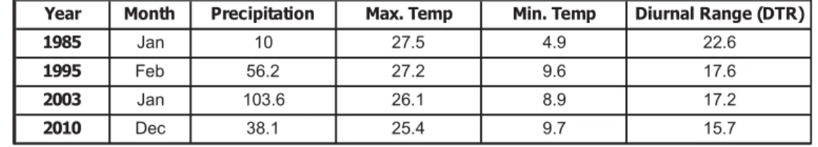
Table 5. 1985, 1995, 2003 and 2010 meteorological data (Kenya Meteorological Department, Narok Station).

LST Change Results and Analysis

LST maps were generated for each of the years of study as depicted in Figure 19 (see the end of this chapter). Apart from that in 2003, increases in the maximum and minimum temperatures occurred in 1985, 1995 and 2010. Issues with cloud cover in the 2003 image may have contributed to the decrease in average temperature. The areas closest to northeastern, central and eastern parts of the study area had the highest temperatures of all the years, whereas the western part had the lowest temperatures. The areas with highest LST were dominated by

Year Month Precipitation Max. Temp Min. Temp Diurnal Range (DTR)

1985 Jan 10 27.5 4.9 22.6

1995 Feb 56.2 27.2 9.6 17.6

2003 Jan 103.6 26.1 8.9 17.2

2010 Dec 38.1 25.4 9.7 15.7

(21)

Table 6. Summary of LULC spatial coverage.

bare earth and cultivated land cover classes. The mean LST in 1985 was 27.9 °C with maximum and minimum LSTs of 35 °C and 16 °C, respectively. In 1995, the mean LST was 27.1 °C, the maximum was 38 °C and the minimum was 18 °C. This trend represents 2 °C and 3 °C increases in minimum and maximum LST, respectively, and a 1 °C increase in diurnal LST range. The minimum and maximum LSTs in 2003 were 8 °C and 28 °C, respectively, for both the low-gain and high-gain images.

The aforementioned results indicate that for the study area, surface brightness had minimal influence on the recorded at-sensor radiance, given that the images were not subjected to atmospheric corrections. The mean LST in 2003 was 17.7 °C, representing a significant decrease in comparison to that in 1995, which is attributable to cloud cover and the influence of precipitation events in January 2003. The minimum LST as derived from the December 2010 image was 20 °C, and the maximum LST was 40 °C, with an average temperature of 29.4 °C. As

YEAR LAND COVER CLASS AREA (km²) COVERAGE %

Water 18.32 0.283

Forests/Dense Vegetation 251.99 3.897

Grasslands/Sparse Vegetation 1760.8 27.232

Bare Earth 4238.25 65.547

Water 28.28 0.437

Bare Earth 3348.69 51.789

Water 42.9 0.663

Bare Earth 2939.93 45.467

Water 36.79 0.569

Bare Earth 2487.92 38.477

1985

1995

2003

2010

(22)

shown in Table 5, the satellite-derived LST information depicted similar trends as those of the ground meteorological measurements of land surface air temperature recorded by the Narok weather station, in which a progressive and significant increase was noted in the minimum temperature. However, the ground measurements indicated a decrease in the maximum temperature, thus leading to a decreasing diurnal temperature range (DTR) contrary to the satellite-derived LSTs.

These results indicate a nearly commensurate increase in maximum LST and DTR, which may be attributed to LULCC because LST includes the influence or contributions of various land cover types and spatial heterogeneity. The meteorological data was derived from one station and is hence insufficient for making a generalization over the study area.

Shown in Figure 20 (see the end of this chapter), LST change maps were generated to gain further insight into the nature of LST change in the epochs of study in the study area. The LST image maps indicate that most of the study area experienced a temperature decrease between 1985 and 1995, particularly in the regions showing changes in vegetation cover. However, some increase occurred in temperature, particularly in the areas with LULC conversion to bare earth or cultivated land (Figures 17 and 20; see the end of this chapter). The LST changes between the 1995 and 2003 images indicate a substantial decrease in LST over most of the study area, which is also attributable to influence of cloud cover in the 2003 image. The LST changes between the 2003 and 2010 images show a general increase over most of the study area. Table 7 provides a summary of the LST changes between the epochs of study.

Table 7. Land surface temperature changes occurring from 1985 to 1995.

CHANGE PERIOD CHANGE TYPE Area (km²) % CHANGE

Increase 1318.19 20.4

Some Increase 269.84 4.2

Decrease 2891.25 44.7

No change 1986.75 30.7

Increase 7.74 0.1

No Change 0 0

Decrease 6458.28 99.9

Increase 1198.78 18.5

Some Increase 4750.07 73.5

Decrease 0.02 0

No Change 517.15 8

1985–1995

1995–2003

2003–2010

(23)

N ormalized Difference Vegetation Index

The NDVI was derived for each year of study, the data of which was used to generate NDVI maps (Figure 21; see the end of this chapter). The minimum NDVI for the 1985 image was –0.070423, and the maximum NDVI was 0.69048.

The highest NDVI values occurred in the areas under forest or dense vegetation cover, whereas the least NDVI values occurred in the areas of the water class. For the 1995 image, the NDVI values ranged from a minimum of –0.074074 to a maximum of 0.71014, and the mean NDVI was 0.166. These results represent a 0.033 decrease between the two epochs. The 2003 image had the highest minimum NDVI of 0.050943 and the lowest maximum NDVI of 0.62069. This image also had the lowest mean NDVI of 0.116. The 2003 NDVI data may be attributed to precipitation which increased the amount of surface water because 2003 had the highest water coverage (Table 6) and cloud cover effects. The minimum NDVI for the 2010 image was 0.23944, whereas the maximum was 0.71951 and the mean was 0.18.

NDVI change evaluation for each year of study was conducted, and maps depicting the changes between the images were generated. The increase in NDVI was the greatest between the 1985 and 1995 images with a 57.9% increase over the study area, whereas the greatest decrease at 41.8% was observed between the 1995 and 2003 images. These changes may be attributed to land cover change. The conversion of land cover to vegetation was the greatest between the 1985 and 1995 images and was the least between the 1995 and 2003, at which time the conversion of land cover to bare earth was greater than that in other epochs.

Visual inspection of the NDVI change images also reveals that, in the northeastern part of the study area which showed a progressive conversion of land use to agricultural use, there was a continued decrease in NDVI in the epochs of 1995 to 2003 and 2003 to 2010.

Table 8. Changes in NDVI between 1985 and 1995.

NDVI CHANGE

1985–1995 AREA (mi²) AREA (km²) % CHANGE

Increase 1445.77 3744.54 57.9

Decrease 704.95 1825.81 28.2

No Change 345.81 895.65 13.9

6466.01 100

(24)

Figure 23 (see the end of this chapter) and Tables 11, 12 and 13 provide summaries of the NDVI change trends and types.

LST and N DVI Correlation

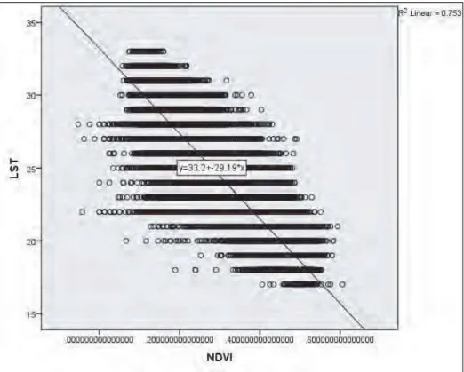
Scatter plots were generated and correlation statistics were computed to investigate the relationship between LST and NDVI for each year of study in the study area. The 1985 LST–NDVI scatter plot reveals a linear negative correlation.

Furthermore, a high degree of correlation was noted, given that R2 is 0.753, which indicates that approximately 75% of the variations in LST were influenced or may be explained by NDVI.

A Pearson two-tailed correlation was then computed for LST and NDVI, as shown in Figure 25. A high degree of association was noted between LST and NDVI (r = 0.868), which differs significantly from 0 (P < 0.001).

NDVI CHANGE

Increase 602.32 1560 24.1

Decrease 1043.62 2702.96 41.8

No change 850.6 2203.05 34.1

Total 6466.02 100

NDVI CHANGE

Increase 1023.74 2651.49 41

Decrease 482.36 1249.31 19.3

No change 990.43 2565.22 39.7

Total 6466.02 100

(25)

Figure 24. 1985 land surface temperature–normalized difference vegetation index (LST–NDVI) scatter plot.

Figure 25. 1985 LST–NDVI correlation.

The trend line for the 1995 image also shows a negative correlation between LST and NDVI with a relatively high degree of linearity (R2 = 0.718).

LST NDVI

Pearson

Correlation 1 0.868^**

Sig. (two-tailed) 0

N 149669 149669

Pearson

Correlation 0.868^** 1

Sig. (two-tailed) 0

N 149669 149669

Correlations

LST

NDVI

** Correlation is significant at the 0.01 level (two-tailed test).

(26)

Figure 26. 1995 LST–NDVI scatter plot.

A Pearson two-tailed correlation of the 1995 LST and NDVI values shows a high degree of association between LST (r = –0.847) with approximately 71% of LST variations probably attributed to NDVI.

Figure 27. 1995 LST–NDVI correlation.

NDVI LST

Pearson

Correlation 1 0.847**

Sig. (two-tailed) 0

N 149669 149669

Pearson

Correlation 0.847** 1

Sig. (two-tailed) 0

N 149669 149669

Correlations

NDVI

LST

** Correlation is significant at the 0.01 level (two-tailed test).

(27)

The 2003 scatter plot and correlation reveal a low degree of negative correlation and association between LST and NDVI (R² = 0.020), which indicates that only approximately 2% of LST variations may be attributed to NDVI.

LST and NDVI were also weakly associated and correlated in the 2010 image, although a negative linear correlation remained.

Approximately 45% of LST variations in 2010 may be explained by NDVI.

Wildlife Data

The wildlife data acquired from DRSRS was not amenable to GIS because of a lack of spatial dimension in the data; however, a qualitative analysis of the data was conducted. Table 11 and Figure 31 (see the end of this chapter) provide summaries of the livestock and wildlife count data in the years of study ± one year.

Large herbivorous mammal species and cattle were selected for the qualitative analysis because they are most affected by environmental changes that result in loss of vegetation.

(28)

The livestock and wildlife counts indicate a major decrease in wildlife populations, particularly those of large mammals. Wildebeests are the flagship species for the MMNR, and their annual migration has earned the MMNR the distinction of being a World Wonder and a major tourist attraction. Apart from vegetation loss, this species is also affected by habitat fragmentation such as that

Figure 30: 2010 LST–NDVI correlations

(29)

Table 11. Wildlife and livestock count data for 1985, 1994, 2004 and 2011.

created by roads, human settlements and poaching. Elephants have long been poached for their tusks, and their numbers dramatically reduced from 2,037 in 1985 to 1,806 in 1994 in the MMNR. Although the population increased to 4397 in 2004 perhaps due to anti-poaching campaigns, it decreased to 3,388 by the following animal count in 2011. This decrease may be attributed to factors such as drought resulting in loss of vegetation, accelerated human–wildlife conflicts due to land use change and competition for grazing resources with livestock. Moreover, elephants can travel great distances and are therefore likely to migrate to other more conducive areas in the face of adversity.

The effects of drought on livestock and wildlife in the MMNR are evident in the animal count data. The significant decrease in the population of all wildlife species and livestock counted in Narok and Trans Mara in 1994 may have been the first indication of the widespread 1995–1996 drought. The 2010 drought also

YEAR SPECIES NO. (population estimate)

Cattle 716,516

Buffalo 20,832

Elephant 2,037

Zebra 78,044

Wildebeest 62,314

Cattle 569,856

Buffalo 5,617

Elephant 1,806

Zebra 50,805

Wildebeest 32,165

Cattle 774,580

Buffalo 419685

Elephant 4,397

Zebra 53,486

Wildebeest 30,651

Cattle 630,103

Buffalo 5,910

Elephant 3,388

Zebra 62,379

Wildebeest 256,507

1985

1994

2004

2011

(30)

devastated the animal populations, and wildlife distribution maps generated from the 2011 animal count show concentrations of wildlife within the MMNR where water reserves are usually the last to be depleted in the event of drought because of limitation of human activities within the reserve. The migratory wildlife of the MMNR is usually dispersed in the surrounding rangelands during the dry season, and there is a substantial number of year-round wildlife residing in the rangelands.

4. Conclusions and Recommendations

I’m no longer sceptical. I no longer have any doubt at all. I think climate change is the major challenge facing the world.—Sir David Attenborough.

(Sir David Attenborought)

This study incorporates the use of a remote sensing approach and statistical and qualitative analysis to investigate the LST, NDVI and LULCC trends, interrelationships and effects on wildlife and livestock. The chosen study area encompasses the MMNR and is bounded by the towns of Ang’ata, Lolgorian, Kilgoris, Lemek, Narok, Maji Moto and Olposumoru and trading centres in Narok and Trans Mara districts. The years of study include 1985, 1995, 2003 and 2010.

Satellite images and ancillary data including meteorological data from the Narok meteorological station, topographic maps and wildlife data have been acquired.

Satellite imagery specifically includes the DJF season, which is typically a dry season for the region and hence exhibits less cloud cover. The satellite imagery used includes multispectral Landsat TM and ETM+ , with a spatial resolution of 30 m in all bands apart from Band 6, which has spatial resolutions of 120 m for the TM data and 60 m for the ETM+ data. LST and NDVI were derived for each image, and correlation analysis was conducted. LULC maps were also prepared for each year. Change detection and analyses for LULC, LST and NDVI were conducted between the study epochs.

LULC maps show that the study area is dominated by bare land and grasslands and sparse vegetation for all epochs. However, while dominant as a land cover, the area of land under bare earth consistently decreased in all epochs while that under grasslands increased. The area of land under cultivation also increased in all epochs apart from 1995 to 2003. However, this decrease may be attributed to the fact that in 2003, most of the cultivated land had crops. This result is uncharacteristic of the region because the DJF season is normally dry and does not support planting. This may therefore be an indication of a change in land use regime caused by above-normal precipitation, as was the case in January 2003 when the mean precipitation recorded at the Narok meteorological station was

(31)

103.6 mm. Farmers in the area rely on rainfall rather than irrigated farming.

Therefore, the presence of crops in 2003 may be an indication of a change in farm operations and farmer behaviour in which planting occurred at an unusual time. In 2003, the area of land under water also increased, which is shown by the increase in detected land surface water in the 1995 to 2003 epoch and the decrease between 2003 and 2010. This may also be attributed to high levels of precipitation leading to water being trapped in crevices and seasonal rivers, as shown in the LULC maps.

Change detection and analysis for the LULC maps also showed an increase in forest/ dense vegetation in the 1995 to 2003 epoch. Given that one of the major problems facing the environment and climate in Kenya is deforestation, this increase may be the result of increase in dense vegetation and not forest coverage.

Furthermore, while it is possible to reclaim forest cover through activities such as reforestation, the available data were insufficient to aid in the identification of new forest cover.

Table 12: Percentages of land use/land cover change (LULCC).

Satellite-derived LST indicated more decrease than increase in LST over the study area for all land covers in all epochs apart from that in 2003. However, the

LULCC % CHANGE

1985 1995 water change 54.36681223

1985 1995 forest/dense vegetation change 9.44878765 1985 1995 grasslands/sparse vegetation change 39.22535211

1985 1995 bare earth change 20.98885153

1985 1995 cultivated land change 83.97070789

1995 2003 water change 51.69731259

1995 2003 forest change 55.24292966

1995 2003 grasslands change 13.79411621

2003 2010 water change 14.24242424

2003 2010 forest change 29.9444133

2003 2010 grasslands change 14.20039862