Wideband phase‑locked loop circuit with real‑time phase correction for frequency modulation atomic force microscopy
著者 Fukuma Takeshi, Yoshioka Shunsuke, Asakawa Hitoshi
journal or
publication title
Review of Scientific Instruments
volume 82
number 7
page range 73707
year 2011‑07‑01
URL http://hdl.handle.net/2297/29300
doi: 10.1063/1.3608447
Wideband phase-locked loop circuit with real-time phase correction for frequency modulation atomic force microscopy
Takeshi Fukuma,1,2,3,a)Shunsuke Yoshioka,2and Hitoshi Asakawa3
1Frontier Science Organization, Kanazawa University, Kakuma-machi, Kanazawa 920-1192, Japan
2Division of Electrical and Computer Engineering, Kanazawa University, Kakuma-machi, Kanazawa 920-1192, Japan
3Bio-AFM Frontier Research Center, Kanazawa University, Kakuma-machi, Kanazawa 920-1192, Japan (Received 20 April 2011; accepted 16 June 2011; published online 20 July 2011)
We have developed a wideband phase-locked loop (PLL) circuit with real-time phase correction for high-speed and accurate force measurements by frequency modulation atomic force microscopy (FM- AFM) in liquid. A high-speed operation of FM-AFM requires the use of a high frequency cantilever which, however, increases frequency-dependent phase delay caused by the signal delay within the cantilever excitation loop. Such phase delay leads to an error in the force measurements by FM- AFM especially with a low Q factor. Here, we present a method to compensate this phase delay in real time. Combined with a wideband PLL using a subtraction-based phase comparator, the method allows to perform an accurate and high-speed force measurement by FM-AFM. We demonstrate the improved performance by applying the developed PLL to three-dimensional force measurements at a mica/water interface.© 2011 American Institute of Physics. [doi:10.1063/1.3608447]
I. INTRODUCTION
Frequency modulation atomic force microscopy (FM- AFM)1has widely been used for atomic-scale studies on var- ious materials in vacuum.2,3 In addition, recent advances in FM-AFM instrumentation4has enabled its operation in liquid with true atomic resolution,5which has stimulated subsequent studies on biological systems by FM-AFM.6–10However, bi- ological systems have much larger fluctuations, corrugations, and inhomogeneity than those of the typical samples that have been studied by FM-AFM in vacuum. Therefore, non- destructive imaging of biological systems requires to enhance the operation speed of FM-AFM. Although molecular-scale imaging of relatively simple biological systems have been realized even with a present FM-AFM system,6–10 a large part of the biological systems and phenomena have remained inaccessible by FM-AFM due to the insufficient operation speed.
The improvement of the operation speed in FM-AFM re- quires to enhance the resonance frequency or the bandwidth of each component constituting the tip-sample distance feed- back loop. In particular, the enhancement of the cantilever resonance frequency (ω0≡2πf0) is essential as it determines the theoretical limit of the operation speed and the force sen- sitivity in FM-AFM.1 Owing to the recent progress in the micromachining technologies, small cantilevers with a mega- hertz order f0 has become commercially available. In con- trast, knowledge on the instrumentation and techniques re- quired for using such a high frequency cantilever has not been established especially for the FM-AFM operation in liquid.
In FM-AFM, the cantilever excitation frequency (ω≡ 2πf) is regulated with a feedback control circuit such that
a)Electronic mail: [email protected].
the phase difference between the cantilever excitation and the deflection signals is kept constant. This feedback control op- erates based on the assumption that the frequency-dependent phase change in the frequency range around f0is caused only by the cantilever. However, in the case of FM-AFM with a low Q factor and a high frequency cantilever, the frequency- dependent phase delay (φd) caused by the other components in the feedback loop is not necessarily negligible, which leads to an error in the measurements of conservative and dissipa- tive forces by FM-AFM.11,12
Recently, it has become common to use a phase-locked loop (PLL) circuit for producing a cantilever excitation sig- nal as well as for the detection of the frequency shift (f) of the cantilever oscillation in FM-AFM.13In the previous study, we have presented a design for a high-speed digital PLL with a subtraction-based phase comparator (S-PLL).14 The devel- oped S-PLL has a detection bandwidth of 100 kHz, which is much higher than that of a commonly used digital PLL with a multiplication-based phase comparator (M-PLL). However, accurate cantilever excitation with the S-PLL has remained difficult mainly due to the error caused byφd. In addition, the effects of the improved operation speed obtained by the S- PLL has not been experimentally demonstrated in FM-AFM measurements.
In this study, we have developed a digital S-PLL with a real-time phase correction circuit for an accurate cantilever excitation and a high-speedf detection. First, we describe the mechanism causingφd in FM-AFM. Second, we pro- pose to combine a real-time phase correction circuit with an S-PLL to compensate φd. Third, we demonstrate the ef- fect of the phase correction circuit by comparing the phase versus frequency curves obtained by PLLs with different de- signs. Finally, we demonstrate the improved performance of the developed S-PLL in a high-speed measurement of three- dimensional force distribution at a mica/water interface.
0034-6748/2011/82(7)/073707/5/$30.00 82, 073707-1 © 2011 American Institute of Physics
073707-2 Fukuma, Yoshioka, and Asakawa Rev. Sci. Instrum.82, 073707 (2011)
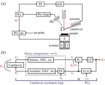
FIG. 1. (Color online) (a) Typical experimental setup for FM-AFM.
(b) Simplified model of a cantilever excitation circuit used in FM-AFM.
II. FREQUENCY-DEPENDENT PHASE DELAY
In this section, we describe the mechanism causingφd
in an FM-AFM setup to clarify the problem to be solved in this study. Figure1(a)shows a typical FM-AFM setup using a PLL for the cantilever excitation. In this setup, a cantilever deflection signal is fed into a PLL which producesf and cantilever excitation signals. The phase and amplitude of the excitation signal is adjusted by a phase shifter (PS) and an automatic gain control (AGC) circuit, respectively, before it is applied to an actuator to drive a cantilever. Hereafter, we refer to the loop consisting of a cantilever, a pre-amp, a PLL, a PS, an AGC and an actuator as “the cantilever excitation loop.”
Figure1(b)shows a schematic diagram of the cantilever excitation loop and the PLL. The PLL consists of a phase comparator (PC), a loop filter (LF), and a voltage controlled oscillator (VCO). Among them, the PC is shared with the can- tilever excitation loop while the LF and the VCO are imple- mented outside. The PC compares the phase of the PLL input (va) and the VCO output (vb) signals and outputs their differ- ence (φPC). This signal is filtered by the LF and fed into the VCO which outputs a sine wave whose frequency (ω) changes in proportion to the input signal (ω) with an offset frequency ofω0(i.e.,ω=ω0+ω). The VCO output is routed back to the PC. This loop works to adjustωsuch thatφPCis kept con- stant. As a result,ωis regulated to equal the frequency of the PLL input.
In the basic principle of FM-AFM, ω is adjusted to keep the phase delay caused by the cantilever (φCL) at−90◦. Namely, the phase difference betweenvaandvb in Fig.1(b) is kept constant. However, in a typical FM-AFM setup, the phase difference betweenva andvb (i.e.,φPC) is kept con- stant. In the setup, there are several components betweenva andvaand betweenvbandvb such as a cantilever deflection sensor and an actuator for the cantilever excitation. The signal delay caused by these components (τd) leads to a phase delay φdgiven by
φd=τdω=τdω0+τdω≡φ0+φd. (1)
In the right side of this equation, the first term φ0 (≡
τdω0) is constant and hence can be compensated with a PS as shown in Fig. 1(b). In contrast, the second term φd
(≡τdω) varies in proportion toωduring FM-AFM mea- surements, which cannot be compensated with a constant PS.
Owing to the frequency-dependent phase delayφd,φCL is not kept constant and shows deviation from −90◦. As the quantitative interpretation of the conservative and dissipative forces measured by FM-AFM is based on the assumption that φCL is kept at −90◦,15 the variation ofφCL gives rise to an error in such an interpretation.11,12
The influence from φd is particularly serious when a high frequency cantilever is used in liquid.φdincreases with increasingωwhileωincreases with increasingω0. Thus, the use of a high frequency cantilever results in a largeφd. In addition, the Q factor (Q) of the cantilever resonance in liq- uid is much lower than that in air or in vacuum. With a low Q factor,φCL shows small frequency dependence around f0 so that the phase change caused byφdis not negligible. Conse- quently, the influence fromφdis more evident in liquid than that in air or in vacuum.
III. REAL-TIME PHASE CORRECTION
In this section, we present a PLL design that allows to solve the problem caused byφd. We first introduce the de- signs for the cantilever excitation circuits using an M-PLL and an S-PLL. Then, we propose a design for an S-PLL with a real-time phase correction circuit, which enables to compen- sate the frequency-dependent phase change caused byφd.
Figures2(a)and2(b)show designs for the cantilever ex- citation circuits with an M-PLL and an S-PLL, respectively.
In an M-PLL, a multiplication-based PC is used for the de- tection ofφPC, where two input sine waves are multiplied to produce 2ω and DC components. While the 2ω component is suppressed by low pass filter (LPF), the DC component is used as a phase signal. In this design, the use of a LPF in the PLL significantly reduces the PLL bandwidth (BPLL). In contrast, S-PLL is free of this problem owing to the use of a subtraction-based PC, where the phase of the PLL input sig- nal is compared with that of the signal from the phase-output VCO (φ-VCO) by subtraction. Owing to the linear subtrac- tion process, no higher harmonics are generated and hence no LPF is required. Thus, the S-PLL design is more suitable for a high-speedf detection than the M-PLL design.
However, one drawback of the S-PLL design is an in- crease of the delay components in the cantilever excitation loop. In the S-PLL design, non-linear signal processing units such as a phase detector and a cosine wave generator are not implemented in the PLL but in the cantilever excitation loop.
Although this is the major reason for the wide bandwidth ob- tained by this design, these additional delay components in- creaseφd. Therefore, the problem caused byφd is more serious in the S-PLL design than that in the M-PLL design.
To solve this problem, we propose a design for an S-PLL with a real-time phase correction circuit [Fig. 2(c)]. In this design, the PLL output (ω) is multiplied byτd to obtain a signal corresponding toφd(=τdω). The obtained signal is subtracted from the output of the phase detector to cancel
FIG. 2. (Color online) Block diagrams showing the cantilever excitation setups with different PLL designs. (a) M-PLL. (b) S-PLL. (c) S-PLL with a phase correction circuit.
outφd. In this way, the design enables cantilever excitation without the influence fromφd.
Although it is also possible to develop an M-PLL with a phase correction circuit, such a PLL is probably too slow to be used in many of the applications. The phase correction circuit is a feedback loop consisting of a PLL, a multiplier, a LPF, and a PS as shown in Fig.2(c). To ensure the stability of the loop, the cutoff frequency of the LPF (fLPF) should be set at a value sufficiently lower than BPLL. For the developed S-PLL havingBPLLon the order of megahertz, we use fLPFof 10 kHz to ensure the stability. Thus, for a typical M-PLL havingBPLL
on the order of kilohertz, we expect that fLPFshould be set at
∼10 Hz, which is too slow for many of the applications.
IV. EXPERIMENTAL DETAILS
The S-PLLs with and without the phase correction circuit were implemented in a field programmable gate array (FPGA) chip (Virtex-4 SX: Xilinx). 14-bit ADCs (AD6645: Analog Devices) and DACs (AD9772: Analog Devices) were used for the signal conversions. The FPGA, ADCs, and DACs were driven at a clock frequency of 20 MHz.
For the purpose of comparison, we used a commercially available M-PLL (OC4: Nanonis). The ADCs and DACs of this PLL are driven at a clock frequency of 40 MHz, which is twice as high as that for the S-PLL used in this study.
The AFM experiments were performed with a custom- built FM-AFM with a low noise cantilever deflection sen- sor and a photothermal cantilever excitation system.4,16,17A commercially available AFM controller (ARC2: Asylum Re- search) was used with some modifications in the software.
The AFM experiments were performed at room temperature.
The measurements of theφPCversus frequency curves were performed in pure water while the 3D imaging was performed in phosphate buffer saline (PBS) solution. The sample for the 3D imaging was prepared by cleaving a mica disc (01877- MB: SPI Supplies) and depositing 150 μl of PBS solution onto the surface.
V. PHASE VERSUS FREQUENCY CURVES
Figure3(a)showsφPCversus frequency curves measured by the S-PLLs with and without the phase correction circuit.
A band pass filter (BPF) was used as a model of a cantilever
073707-4 Fukuma, Yoshioka, and Asakawa Rev. Sci. Instrum.82, 073707 (2011)
60 30 0 -30 -60
600 650 700
Phase [deg.]
Frequency [kHz]
M-PLL
M-PLL (Qa=7.7)
S-PLL (Qa=6.2) S-PLL
3 2 1 0 -1 -2 -3
642 643 644 645 646
Phase [deg.]
Frequency [kHz]
Calculated
Calculated
Drive Frequency [kHz]
Phase [deg.]
90 0 -90 -180
600 700 800 900
180
With correction fBPF = 732 kHz QBPF = 5
fBPF
f0 = 644 kHz QCL = 6.3
f0 = 644 kHz QCL = 6.3 Without correction (a)
(b) (c)
FIG. 3. (Color online) (a)φPCversus frequency curves measured by the S- PLLs with and without the phase correction circuit. A BPF is used as a model of a high frequency cantilever. (b)φPCversus frequency curves measured by the M-PLL and the S-PLL with the phase correction circuit. The measure- ments were performed in pure water with a high frequency cantilever (Arrow UHF: Nanoworld) (f0=644 kHz andQ=6.3). The cantilever oscillation was excited by the photothermal excitation method (see Ref.17). (c) Magni- fied view of the curves shown in (b).
to obtain an ideal phase versus frequency curve of a second- order resonance. The dotted line in the figure shows an ideal phase curve calculated with the Q factor (QBPF=5) and the center frequency (fBPF=732 kHz) of the BPF. The phase curve measured without the phase correction shows a much larger frequency-dependent phase change compared to that of the ideal phase curve. In contrast, the curve measured with the phase correction shows almost the same profile as that of the ideal one. The results demonstrate thatφdis effectively compensated by the phase correction circuit.
Figure3(b)showsφPCversus frequency curves measured by the M-PLL and the S-PLL with the phase correction cir- cuit. The measurements were performed in pure water us- ing a high frequency cantilever (Arrow UHF: Nanoworld).
The cantilever was excited by the photothermal excitation method17 to obtain an ideal phase versus frequency charac- teristics of a cantilever. The phase curve measured with the M-PLL shows larger frequency-dependent phase delay com- pared to the one obtained with the S-PLL due to the influence fromφd.
A magnified view of these curves around f0is shown in Fig.3(c). The dotted line corresponds to the ideal phase curve calculated with the cantilever parameters f0=644 kHz and Q=6.3, which were estimated by fitting a thermal vibration spectrum of the cantilever in water. The phase curve obtained by the S-PLL shows good agreement with the ideal curve while the one obtained by the M-PLL shows a large devia- tion from it. In principle, an M-PLL is more immune to the φd than an S-PLL. Nevertheless, the result shows that the influence fromφdis not negligible even with an M-PLL.
In the frequency range around f0, a phase curve shows almost linear dependence on the frequency as shown in Fig.3(c). From the slope of a phase curve in this frequency range, an apparent Q factor (Qa) can be calculated based on the following equation:12
Qa= dφ
df f0
2 . (2)
TheQavalues calculated with the phase curves obtained with the M-PLL and the S-PLL are 7.7 and 6.2, respectively. Com- pared to the true Q factor estimated from the thermal vibra- tion spectrum (Q=6.3), these values contain+22.2% and
−1.6% errors, respectively. This result shows that the increase ofQacaused byφdcan be greatly suppressed by the S-PLL with the phase correction circuit. As the increase of Qa di- rectly leads to an error in the interpretation of the measured conservative and dissipative forces, the suppression ofQais essential for an accurate force measurements by FM-AFM.
VI. 3D HYDRATION FORCE MEASUREMENTS
We have performed measurements of 3D force distri- bution at a mica/water interface by 3D scanning force mi- croscopy (3D-SFM) (Ref. 18) using the M-PLL and the S-PLL with the phase correction circuit. In 3D-SFM, the ver- tical tip position (zt) is modulated with a frequency (fm) faster than the bandwidth of the distance regulation while the tip is laterally scanned. During the scan,f is recorded in real time with respect to the 3D tip position while the averaged tip height is regulated to keep the averagedf value constant. In this technique, a high-speed FM detector is required for the real time recording of the f variation induced by the fast modulation of the tip height. Thus, this application is suitable for testing the effect of the enhanced bandwidth obtained by the S-PLL.
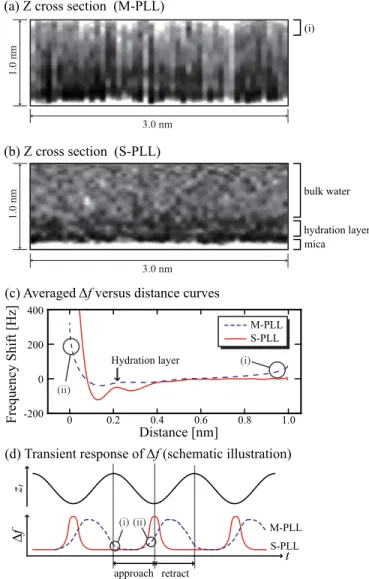
Figures4(a)and4(b)show Z cross sections derived from the 3D f images obtained by the M-PLL and the S-PLL with the phase correction circuit, respectively. The image ob- tained with the S-PLL shows a clearer contrast than that ob- tained by the M-PLL due to the enhanced BPLL. This differ- ence is particularly evident in the contrasts corresponding to a hydration layer. While the image obtained by the S-PLL shows a layer-like contrast near the mica surface, the image obtained by the M-PLL shows a vague and broad contrast at the corresponding position.
This difference is also confirmed in thef versus dis- tance curves [Fig. 4(c)] obtained by averaging the images shown in Figs.4(a)and4(b). The curve obtained with the S- PLL shows a clear peak corresponding to the hydration layer as indicated by the arrow while such a peak is hardly seen in the curve obtained with the M-PLL. These results demon- strate that the S-PLL has an advantage over the M-PLL in the high-speed imaging of 3D hydration structure.
The image obtained by the M-PLL shows a bright con- trast at a region far from the surface [region (i) in Fig.4(a)].
Since this region corresponds to the bulk water, it should show a uniformf distribution as seen in the image obtained by the S-PLL. Thus, the bright contrast found in Fig.4(a)should be a measurement error. Here, we explain the mechanism causing
FIG. 4. (Color online) (a) and (b) Z cross sections derived from the 3Df images obtained at a mica/water interface using (a) the M-PLL and (b) the S-PLL with a phase correction circuit. fm=781 Hz. Spring constant: 12.9 N/m. Oscillation amplitude: 0.19 nm (M-PLL) and 0.48 nm (S-PLL).Q= 6.1. 13 s per 3D image (82 ms per XZ image). (c)f versus distance curves obtained by averaging the Z cross sections shown in (a) and (b). (d) Schematic illustration showing the transient response off signal during the 3D-SFM measurements.
this error with the schematic illustration showing the transient response off during the 3D-SFM imaging [Fig.4(d)].
During the 3D-SFM imaging,ztis modulated with a sine wave as shown in Fig.4(d). In response to the tip approach and retract,f should show a sharp increase and decrease near the sample surface, respectively. Thus, if the PLL re- sponse is sufficiently fast, the f signal should change as illustrated by a solid line in Fig.4(d). However, if the PLL response is too slow, thef signal may exhibit a significant delay as illustrated by a dotted line in Fig.4(d).
As the images shown in Figs.4(a)and4(b)were obtained by recording thef signal during the tip approach processes, the transientf response indicated by circles (i) and (ii) in Fig.4(d)should lead to an error in the obtained image and the force curve. In fact, the bright contrast found in region (i) in Fig.4(a)corresponds to the error indicated by circle (i) in
Fig.4(d). This error is also confirmed in the force curve shown in Fig.4(c)as indicated by circle (i). Similarly, the error in- dicated by circle (ii) in Fig.4(d)accounts for the delayedf response indicated by circle (ii) in Fig. 4(c). These results demonstrate that the improvedBPLLobtained by the S-PLL is essential for an accurate and high-speed force measurement by FM-AFM in liquid.
Although the imaging speed of 3D-SFM is not deter- mined only by BPLL, here we describe the improvement that we observed in the case of our experimental setup. With the setup using the M-PLL, the fastest imaging speed that allows to obtain an image without a significant distortion was 53 s per 3D image (fm=200 Hz, 0.32 s per XZ image) as reported previously.12 With the developed S-PLL using the real-time phase correction circuit, we have been able to obtain a 3D im- age in 13 s (fm=781 Hz, 0.082 s per XZ image) as shown in Fig.4(b). This is an improvement by a factor of four. In addition, the present imaging speed is not limited by the PLL bandwidth but by the data acquisition speed. As the devel- oped PLL has BPLL higher than 100 kHz, we expect that it should allow imaging with fm higher than a few kilohertz.
This corresponds to the imaging speed faster than 10 s per 3D image.
ACKNOWLEDGMENTS
This work was supported by PRESTO, Japan Science and Technology Agency.
1T. R. Albrecht, P. Grütter, D. Horne, and D. Ruger,J. Appl. Phys.69, 668 (1991).
2Noncontact Atomic Force Microscopy (Nanoscience and Technology) edited by S. Morita, R. Wiesendanger and E. Meyer (Springer-Verlag, Berlin, 2002).
3Noncontact Atomic Force Microscopy (Nanoscience and Technology) edited by S. Morita, R. Wiesendanger, and F. J. Giessibl (Springer-Verlag, Berlin, 2009) Vol. 2 .
4T. Fukuma, M. Kimura, K. Kobayashi, K. Matsushige, and H. Yamada, Rev. Sci. Instrum.76, 053704 (2005).
5T. Fukuma, K. Kobayashi, K. Matsushige, and H. Yamada,Appl. Phys.
Lett.87, 034101 (2005).
6B. W. Hoogenboom, H. J. Hug, Y. Pellmont, S. Martin, P. L. T. M. Frederix, D. Fotiadis, and A. Engel,Appl. Phys. Lett.88, 193109 (2006).
7M. Higgins, M. Polcik, T. Fukuma, J. Sader, Y. Nakayama, and S. P. Jarvis, Biophys. J.91, 2532 (2006).
8T. Fukuma, A. S. Mostaert, and S. P. Jarvis,Nanotechnology19, 384010 (2008).
9H. Yamada, K. Kobayashi, T. Fukuma, Y. Hirata, T. Kajita, and K. Mat- sushige,J. Appl. Phys.2, 103703 (2009).
10K. Nagashima, M. Abe, S. Morita, N. Oyabu, K. Kobayashi, H. Yamada, M. Ohta, R. Kokawa, R. Murai, H. Matsumura, H. Adachi, K. Takano, and S. Murakami,J. Vac. Sci. Technol. B28, C4C11 (2010).
11G. B. Kaggwa, J. I. Kilpatrick, J. E. Sader, and S. P. Jarvis,Appl. Phys.
Lett.93, 011909 (2008).
12T. Fukuma,Sci. Technol. Adv. Mater.11, 033003 (2010).
13U. Dürig, H. R. Steinauer, and N. Blanc,J. Appl. Phys.82, 3641 (1997).
14Y. Mitani, M. Kubo, K. Muramoto, and T. Fukuma,Rev. Sci. Instrum.80, 083705 (2009).
15J. E. Sader, T. Uchihashi, M. J. Higgins, A. Farrell, Y. Nakayama, and S. P.
Jarvis,Nanotechnology16, S94 (2005).
16T. Fukuma and S. P. Jarvis,Rev. Sci. Instrum.77, 043701 (2006).
17T. Fukuma,Rev. Sci. Instrum.80, 023707 (2009).
18T. Fukuma, Y. Ueda, S. Yoshioka, and H. Asakawa,Phys. Rev. Lett.104, 016101 (2010).