Asymptotic cumulants of some information criteria Haruhiko Ogasawara

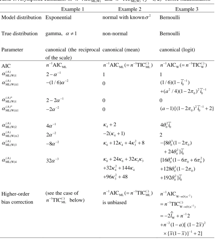
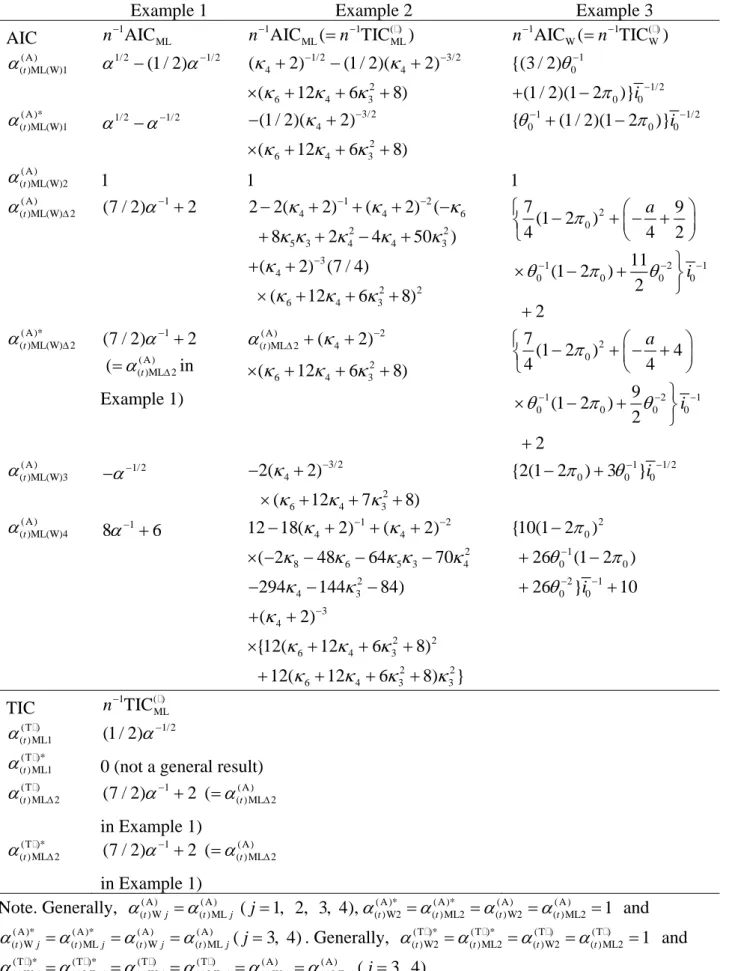
No.170

Asymptotic cumulants of some information criteria

Haruhiko Ogasawara

April 2015

Department of Information and Management Science

Otaru University of Commerce

Discussion Paper, No.170, April, 2015, Center for Business Creation, Otaru University of Commerce, Otaru, Japan.

Asymptotic cumulants of some information criteria

Haruhiko Ogasawara Otaru University of Commerce

This work was partially supported by a Grant-in-Aid for Scientific Research from the Japanese Ministry of Education, Culture, Sports, Science and Technology, No.23500341.

Author’s address: Department of Information and Management Science, Otaru University of

Commerce, 3-5-21, Midori, Otaru 047-8501, Japan. Email: [email protected]

Asymptotic cumulants of some information criteria

Asymptotic cumulants of the Akaike and Takeuchi information criteria are given under possible model misspecification up to the fourth order with the higher-order asymptotic variances, where two versions of the latter information criterion are defined using observed and estimated expected information matrices. The asymptotic cumulants are provided before and after studentization using the parameter estimates by the weighted score method, which include the maximum likelihood and Bayes modal estimators as special cases.

Higher-order bias corrections of the criteria are derived using log-likelihood derivatives, which yields simple results for cases under canonical parametrization in the exponential family. The results are illustrated by three examples.

Keywords: Akaike information criterion; Takeuchi information criterion; Kullback-Leibler

distance; canonical parameters; higher-order bias correction.

1. Introduction

Typical information criteria are given by Akaike (1973) and Takeuchi (1976), which are called the Akaike information criterion (AIC) and Takeuchi information criterion (TIC), respectively. The criteria are used to assess the goodness of statistical models based on the Kullback-Leibler (1951) distance using the maximum likelihood estimators (MLEs) of associated parameters. In the AIC, it is assumed that a posited model holds or that a true model is a special case of the model employed. On the other hand in the TIC, possible model misspecification is considered. Stone (1977) derived the TIC in the context of cross validation. Linhart and Zucchini (1986, Proposition 2, Appendix A.2.1) also derived the TIC. For properties of the TIC, see Shibata (1989).

After the AIC and TIC were coined, information criteria with similar purposes have been introduced by e.g., Schwarz (1978; the Bayesian information criterion, BIC); Kishino and Hasegawa (1989), Ishiguro, Sakamoto and Kitagawa (1997; the extended information criterion, EIC), Shimodaira and Hasegawa (1999) for the methods using the bootstrap;

Shibata (1989; the regularization information criterion, RIC) and, Konishi and Kitagawa (1996; the generalized information criterion, GIC; see also Konishi & Kitagawa, 2003; 2008, Chapters 5 to 8). In the RIC and GIC, the exclusive usage of the MLEs by the AIC and TIC was relaxed to cover e.g., robust and ridge-type estimators. For other information criteria, see Konishi and Kitagawa (2008) and Burnham and Anderson (2010).

The above information criteria are seen as point estimators of a corresponding

population quantity with bias correction under correct model specification for the AIC and under possible model misspecification for the TIC, RIC and GIC. The population quantity is the so-called mean expected log-likelihood (Sakamoto, Ishiguro & Kitagawa, 1986,

Equation (4.9)) associated with the Kullback-Leibler distance, where independent two-fold expectation is used one for data in the future for prediction and the other for current data for estimation with the same sample size denoted by n. When n increases, the population value increases proportionately in an asymptotic sense. On the other hand, the terms of bias correction are of order O(1) for the AIC and O

_p

(1) for the TIC, RIC and GIC. For tractability, divide the information criteria by n yielding quantities per observation as

1

AIC

n

^

and n

^1

TIC . Then, the population value mentioned above is written symbolically

as O (1)  O n (

^1

) depending on n. The situation is somewhat different from that of typical parameter estimators as MLEs, where the population parameters usually do not depend on n.

When n becomes infinitely large, the population value O (1)  O n (

^1

) for e.g., n

^1

AIC becomes O(1), which is the expected log-likelihood averaged over observations, where the parameters are evaluated by their population values followed by expectation. The last population value of order O(1) is also of interest as well as that of O (1)  O n (

^1

) .

The bias correction of the TIC was extended to the higher-order version by Konishi and Kitagawa (2003), which gives a refined point estimator of the population counterpart.

On the other hand, statistical testing of the difference of the information criteria for different models have been developed by Steiger, Shapiro and Browne (1985) and Shimodaira (1997) under local alternatives and by Linhart (1988), and Kishino and Hasegawa (1989) under fixed alternatives. Interval estimation of the corresponding population quantities can also be done in similar manners. While the above methods of testing and estimation is for general models, the results for special models are available for the higher-order bias correction by Sugiura (1978) and Yanagihara, Sekiguchi and Fujikoshi (2003) and the asymptotic cumulants for standardized estimators by Yanagihara and Ohmoto (2005).

One of the purposes of this study is to derive general expressions of the higher-order bias corrections of n

^1

AIC and n

^1

TIC based on the parameter estimators by the weighted score method under possible model misspecification, where the expression is different from that of Konishi and Kitagawa (2003). The expression is given by the log-likelihood derivatives, which yields some transparent results for e.g., the cases of the natural exponential family. Note that Konishi and Kitagawa (2003) used the von Mises calculus (von Mises, 1947; Withers, 1983).

The second purpose is to give general formulas for the asymptotic cumulants of

1

AIC

n

^

and n

^1

TIC up to the fourth order and the higher-order asymptotic variances before and after studentization for testing and interval estimation of the population

quantities of interest. Three examples using basic distributions in statistics are shown. The

2. The higher-order asymptotic biases

Let θ be a q  1 vector of parameters in a statistical model with a p  1 vector x

^*

of observable variables. Then, the log-likelihood of θ based on n i.i.d. observations is denoted by

* * *

1 1

( | ) log ( | ) ( | )

n n

j j

j j

l l l f f

 

 ^{θ X}     ^{x θ}  ^{X θ} , (2.1) where X

^*

is a n  p matrix whose rows ( x

^*_j

', j  1,.., ) n are independent copies of x

^*

or their realizations for simplicity of notation, and f ( x

^*_j

| ) θ is the probability density/mass function for a posited statistical model. The log-likelihood averaged over observations is denoted by l  n l

^1

. Define

* * *

ML ML ML

ˆ ( ˆ | ) { ( ) | }

l  l θ X  l θ X X , (2.2) where θ ˆ

_ML

is the MLE of the corresponding population quantity θ

₀

. Let θ ˆ

_W

be the vector of the parameter estimators by the weighted score method (WSEs) or the solution of

θ satisfying

*

1 *

( | )

l n

^

  

 θ X

q 0

θ , (2.3) where q

^*

 q

^*

( ) θ , a function of θ , is a q  1 weight vector, which becomes the log-prior derivatives in the case of Bayesian estimation but can be other general weights. Define

* * *

W W W

ˆ ( ˆ | ) { ( ) | }

l  l θ X  l θ X X , (2.4) whose special case is θ ˆ

_ML

in (2.2) when q

^*

 0 _{. Let} Z

^*

be an independent copy of X

^*

, where Z

^*

is interpreted as an independent data set in the future with the same sample size as n from the viewpoint of prediction. Define

* *

0

E { (

_g 0

| )}

( )

(

0

| ) ( |

0

) d

l  l θ Z  

R Z

l θ Z g Z ζ Z , (2.5)

where g ( | Z ζ

₀

) is the true density of Z

^*

determined by the parameter vector ζ

₀

_{of an}

appropriate size, and is possibly different from f ( | Z θ

₀

) . Equation (2.5) is to be

interpreted as the corresponding summation when g ( | Z ζ

₀

) is a probability mass.

Similarly, define

*

0

(

0

| )

_p

(1)

l  l θ X  O with E ( )

_g

l

₀

 l

₀^*

(2.6)

and

W^* ( ) W 0 ( ) W ^* 0

ˆ ( ˆ | ) ( | ) d { ( ) | } ( | ) d

_p

(1).

R R

l  

Z

l θ Z g Z ζ Z  

Z

l θ X Z g Z ζ Z  O _(2.7)

It is assumed that

* 1 2 3

W W 1 2

ˆ ˆ

2E (

_g

l l ) n b

^

n b

^

O n (

^

)

     (2.8) holds, where n b

^1 ₁

and n b

^2 ₂

are defined as the asymptotic biases up to order O n (

^2

) of  2l ˆ

_W

whose population counterpart is  2E (

_g

l ˆ

_W^*

)  O (1) for the AIC and TIC with

2

n b

^ 2

being the higher-order added asymptotic bias.

In the following, we obtain an expression of b

₂

different from that of Konishi and Kitagawa (2003) with b

₁

being well known. For the expression, we use the formula of the expansion of θ ˆ

_W

 θ

_W

( X

^*

) given by Ogasawara (2013, Equation (2.1) (see also 2015 for correction); 2014, Equation (2.4)):

1/2

3

1 1 * ( ) ( ) 1 1 * 1 * 2

W 0 0 0 W W 0 ( )

1 3 *

1 1 * ( ) ( ) 1 1 1 * 1 (1) (1)

0 0 0 0

1 0

1 (3) 1 * 1 (1) 2

0 0 0

1 1 * ( ) ( )

0 0

ˆ ( ˆ ˆ ) ( )

'

E ( ){( ) } ( )

p

j j

O n p j

j j

j

g p

j j

j

n n O n

n n

O n

n



     



     



   

 



      

 

       

    



  





θ θ Λ q Λ l L q Λ q

Λ q Λ l Λ MΛ q Λ q Λ l

θ

Λ J Λ q Λ l

Λ q Λ l

1/2

3

1 ( W ) 2

0 ( )

1

( ) ( ),

p p

O n

n



O n

 

 

 ^l

(2.9)

where Λ  E (

_g



²

l /   θ θ ' |

_{θ θ 0}

)  E (

_g



²

l /   θ θ

_{0 0}

')  O (1), q

^*₀

 q

^*

( θ

₀

),

2 2

( ) ( ) / 2

0

ˆ

W ˆ

(1), ( ) ( 1, 2, 3), | ,

ˆ ˆ

j j j

p

l l

O O n

^

j 

_



    

 

^{θ θ}

 

Λ l L

θ θ

0

2 * *

* * 1/2

W W

0 0 0

ˆ ( )

( ), ( ), | ,

'

^p

' '

l O n

^ _

  

    

   

^{θ θ}

q q θ

q q θ M Λ

θ θ θ θ

3 (3)

0 2

0 0

( ') ,

l

_{ }k

 

    

 

J x x x

θ θ  (k times of x),  denotes the Kronecker

product, and ( )

₍ ^1/2₎

Op n^

 indicates that ( )  is of order O n

_p

(

^{1/ 2}

) with other similar expressions.

The term

3

( ) ( ) 0 1

j j



j

^{Λ l} in (2.9) (Ogasawara, 2010, Equation (2.4)) is given from the following expansion:

3

( ) ( ) 2

ML 0 0

1

ˆ

^{j j} _p

( )

j

O n

^



   

θ θ Λ l , (2.10)

(1) (1) 1

0

0

2

(2) (2) 1 1 1 (3) 1

0 0

0 0

2

(3) (3) 1 1 1 1 1 (3) 1

0 0

0 0

,

1 E ( )

2

1 E ( )

2

g

g

l

l l

l l



 

   

 

     

  



 

 

       

 

 

        

Λ l Λ θ

Λ l Λ MΛ Λ J Λ

θ θ

Λ l Λ MΛ MΛ Λ MΛ J Λ

θ θ

2

1 (3) 1 1 1 1 (3) (3) 1

0 0 0

0 0 0

E ( ) 1 { E ( )}

g

2

g

l l l

^{ }



  

 

  



   







 

 Λ J      Λ MΛ       Λ        Λ J  J   Λ   

θ θ θ

2

1 (3) 1 1 (3) 1

0 0

0 0

3

1 (4) 1

0

0

1 E ( ) E ( )

2

1 E ( ) ,

6

g g

g

l l

l

 

   

 

 

           

 

                     

  

     

Λ J Λ Λ J Λ

θ θ

Λ J Λ

θ

4

(4) (1)

0 3 0

0 0 0

2

(2) (2 1) (2 2) 1

0 0 0

0 0

, ,

( ')

'

v '( ) , ( ', ') ' ( ),

' '

^p

l l

l l

O n

 

 

  

 

 

  

     

 

               

J l

θ θ θ

l M l l

θ θ

2 2

(3) 2 (3) (3)

0 0 0

0 0 0

3

0

(3 1) (3 2) (3 3) (3 4) 3/ 2

0 0 0 0

v '( ) , v '( ) , vec '{ E ( )}

' ' '

' '

( ', ', ', ') ' ( ),

g

p

l l l

l

O n

   

 

 

    

       

                 

    

   

  

 

l M M J J

θ θ θ

θ

l l l l

where l

⁽²₀ ^j)

 O (1) ( j  1, 2) _and l

⁽³₀^j)

 O (1) ( j  1,..., 4) are defined implicitly by

2

(2) (2) (2 ) (2 )

0 0

1

j j

j

 



 

Λ l Λ l _and

^{(3) (3)}₀ ^{4 (3 ) (3}₀ ⁾

1

j j

j

 



 

Λ l Λ l _; v '( M )

^{ 2}

 [{v( M )}']

^{ 2}

_; v( )  is the vectorizing operator taking the non-duplicated elements of a symmetric matrix in parentheses; and vec( )  is the vectorizing operator stacking the columns of a matrix sequentially.

Expand  2l ˆ

_W

_and  2l ˆ

_W^*

_as

/2

4

5/ 2

W 0 (1) W 0 ( )

1 0 (1)

ˆ 1 ˆ

2 2( ) 2 {( ) } ( )

! ( ')

^j

p p

p

j

j

O j O n p

j O

l l l O n

j

^

  

  

  

        _θ   ^θ  ^θ  ^(2.11)

and

^/2

4

* * 5/ 2

W 0 (1) W 0 ( )

1 0 (1)

ˆ 1 ˆ

2 2( ) 2 E {( ) } ( )

! ( ')

^{p j}

j

j

O g j O n p

j O

l l l O n

j

^

  

  

    

          _θ     ^θ  ^θ  ^,

respectively. Then, recalling E ( )

_g

l

₀

 l

₀^*

, we have

1/2

2 2

*

W W

3

3

W 0

1 0 0 ( )

2

W 0 W 0 ( )

0 ( )

(3) (3) 3

0 0 W 0

ˆ ˆ

2E ( )

1 ˆ

2E E ( ) ( )

! ( ') ( ')

ˆ ˆ

2E ( ) E {vec '( )( ) }

'

1 E {vec '{ E ( )}( ˆ ) 3

p

g

j j

j

g j g j

j O n

g g O n

O n

g g

l l

l l

j O n l







  

   



 







 

       

 

                  

  

         

  

 _{θ θ} ^{θ θ}

θ θ M θ θ

θ

J J θ θ

2

3 ( )

}

_{O n}

O n ( ),

 





(2.12)

where the term of j = 4 in 

⁴_j1

( )  of (2.11), when the expectation is taken, is absorbed in the remainder term of order O n (

^3

) ; and E ( )

_g



_{O n(} ²₎

indicates that the expectation is taken up to order O n (

^2

) .

Let

0 0

= E

^g

'

l l

n    

   

 

Γ θ θ . When the model is true, Γ =   Λ I

₀

, where I

₀

is the population Fisher information matrix per observation. Under possible model

misspecification, the last three expectations in (2.12) are given as

1 2

2

W 0

0

3

1 1 * ( ) ( ) 1 ( W )

0 0 0

0 1

1 (2) (2)

0

0 0 ( ) 0 ( )

(3) (3) 0

0 ( )

2E ( ˆ )

'

2E ( )

'

2E 2E

' '

2E '

g

j j g

j

g g

O n O n

g

O n

l

l n n

l l l

l

 



  





  

      

  

         

          

   

                        

    

 

            



θ θ θ

Λ q Λ l l

θ

Λ Λ l

θ θ θ

Λ l

θ

₂

1 ( W ) 3

0

0 ( )

2E ( )

g

'

O n

n l O n



 

    

  

    

   

 l 

θ

1 1 2 ( 2 1) 2 ( : , )

, 1 0 0

( A)

( 2 2) 2 (3 1)

( : , ) ( : , , )

, , 1 0 0 0 , 1

0

2 tr( ) 2 ( ) E

( ) E ( )

cov ( , ) 2 cov ,

q

d ab c g ab

a b c d c d

q q

c a b g f ab cd e

a b c a b c a b c d e f

g ab cd ef g ab

e

l l

n n n m

l l l

n

n m m n m l

 

  

 

   

 

 

   

 

  

         

    

        

 

 



 

  

Λ Γ Λ

Λ Λ

0

cov

_{g cd}

,

f

n m l



     

 

 

        

   

 

(2.13)

3

(3 2) (3 3)

( : , , ) ( : , , )

, , 1 ( , , ) 0 , , , , , 1

3

(3) (3 4)

0 ( , , ) ( : , , )

( , , ) 0 , , , 1

( ) cov , ( )

cov ( ) , ( ) ( )

q q

e ab c d g ab de f abc d e

a b c d e c d e c a b c d e f

q

g a b c ef d a b c ab cd ac bd ad bc

d e f d a b c d

ab

n m l

n l

 

      





 

  





  

      

  

        



   

 

Λ Λ

J Λ

*

1 * 1 1

0

, , 1 0 0

(3) 1 * 1 1 3

0 0

(A)

1 2 3 1

1 1 1 1

( ) ( )

( ) cov , tr

'

tr[E ( ){( ) ( )}] ( )

( ) ( 2tr( ), 2 [ ] ),

q

c g bc

a b c a

g

n l m

O n

n b n c O n b c



  



   

   

      

     

   

    



      



A A

Λ q q Λ ΓΛ

θ

J Λ q Λ ΓΛ

Λ Γ

where ( Λ

^{(2 1)}

)

_{( :d ab c, )}

indicates the element of the d-th row and the column corresponding to ( M )

_ab

 m

_ab

(the (a, b)th element of M) and   l / ( θ

₀

)

_c

   l / 

_0c

of Λ

^{(2 1)}

with

( ) 

_c

being the c-th element of a vector with other expressions defined similarly;

1 1 , 1 1 1

( ) ( ), ( ) ( ); cov ( )

q q q q

a

g

a b b a e f e f

      

    is the covariance using the distribution

*

( |

0

) g X ζ ;

3

( , , )

( )

c d e

  is the sum of three symmetric terms with respect to c, d and e; and

( ) ( )

[  ]

A A

is for ease of finding correspondence;

2

W 0

2

1 1 * 1 1

0

0 0

1 (2) (2)

0 0

E {vec '( )( ˆ ) }

E vec '( ) 2( )

2 ( )

g

g

l l

n

l

 

 

   



 

        

                    

 

   

            M θ θ

M Λ q Λ Λ

θ θ

Λ Λ l

θ

2 1 * 2

0

, , 1 0 , , , 1 0 0

( A)

2 (2 1)

( : , )

, , 1 1 ( , ) 0 0

2 ( ) cov , E

2 ( ) cov , cov ,

cov (

q q

bc ac bd

a g ab g ab

a b c c a b c d c d

q q

ac

b de f g ab g de

a b c d e f c f c f

g

l l l

n n m n m

l l

n m n m

n m

  

  

  

 

 



  

   

   

               

 

    

                



 

  

Λ q

Λ

3

(2 2) 3

( : , )

, , , , 1 ( , , ) 0

( A)

2 3

2

, )

2 ( ) cov , ( )

( ),

ab de cf

q

ac

b d e g ab de

a b c d e c d e c

m

n m l O n

n c O n



 



 



 

 



   

        

 

 ^Λ 

(2.14)

(3) (3) 3

0 0 W 0

3

(3) (3) 1 3

0 0

0

2 (3) 3

0 ( , , )

, , , , , 1 0

2 3

3

1 E [vec '{ E ( )}( ˆ ) ] 3

1 E vec '{ E ( )} ( )

3

cov ( ) , ( )

( ),

g g

g g

d q

ad be cf

g a b c ef

a b c d e f d

l O n

n n l O n

n c O n



   



 

 

 

 



 

  

    

 

             

  

      

 



J J θ θ

J J Λ

J

(2.15)

where 

^bc

 ( Λ

^1

)

_bc

. Then, from (2.13) to (2.15),

Theorem 1. Under (2.8) with regularity conditions for (2.9) and (2.10), the asymptotic biases n b

^1 ₁

and n b

^2 ₂

of  2l ˆ

_W^*

up to order O n (

^2

) , based on the WSE θ ˆ

_W

derived by the estimation equation of (2.3), are given by

*

W W

1 1 2 3 1 2 3

1 2 3 1 2

ˆ ˆ

2E ( )

2tr( ) ( ) ( ) ( ),

g

l l

n

^{ }

n

^

c c c O n

^

n b

^

n b

^

O n

^

 

 Λ Γ        (2.16)

where c c

₁

,

₂

and c

₃

are obtained by (2.13) to (2.15), respectively.

From (2.13) to (2.15), we find that b

₁

and c

₃

do not depend on q

^*₀

_{and are}

common to the results by the MLE θ ˆ

_ML

and the WSE θ ˆ

_W

_while c

₁

and c

₂

depend on

*

q

0

. A considerably simplified result is obtained in the following case.

Corollary 1. When the vector of canonical parameters in the exponential family of distributions is used under possible model misspecification,

* 1 2 3

W W 1 1

ˆ ˆ

2E (

_g

l l ) n b

^

n c

^

O n (

^

)

     _with b

₂

 c

₁

_and c

₂

  c

₃

0 , (2.17) where c

₁

is simplified as

1 1

W 0

0

2 ( 2 2) 2

( : , )

, , 1 0 0 0

( A)

(3 4)

( : , , ) , , , 1

*

1 1 (3) 1 *

0 0

0

2E ( ˆ ) 2 tr( )

'

2 ( ) E

( ) ( )

tr tr[E ( ){( ) (

'

g

q

c a b g

a b c a b c

q

d a b c ab cd ac bd ad bc

a b c d

g

l n

l l l

n n

  

     

 

 







   

  

       

 

   

         

  

  

       





θ θ Λ Γ

θ

Λ

Λ

q Λ ΓΛ J Λ q Λ

θ

1 1 3

( A)

1 2 3

1 1

)}] ( )

( ).

O n n b n c O n

 

  

 

 

  

ΓΛ

(2.18)

Proof. Under canonical parametrization in the exponential family, it is known that

0 0

E ( 2, 3,...)

( ) ( )

j j

j g j

l l

   

j

 

     

 θ   θ  , which gives c

₁

of (2.18) from (2.13) with M = O and J

⁽³⁾₀

 E (

_g

J

⁽³⁾₀

)  O . The results of c

₂

  c

₃

0 are derived similarly from (2.14) and (2.15) with M = O and J

⁽³⁾₀

 E (

_g

J

⁽³⁾₀

)  O , respectively. Q.E.D.

In the case of the MLE, the two terms associated with q

^*₀

in (2.18) vanish and

recalling (2.10) for Λ

^{(2 2)}

and Λ

^{(3 4)}

in c

₁

of (2.18), we have

(2 2) 2

1 ( : , )

, , 1 0 0 0

(3 4)

( : , , ) , , , 1

1 (3) 1 2 2

0

, , 1 ( : , ) 0 0 0

1

2 ( ) E

( ) ( )

2 1 ( ) E

2 1 ( ) 2

q

c a b g

a b c a b c

q

d a b c ab cd ac bd ad bc

a b c d q

g

a b c c a b a b c

l l l

c n

l l l

n

  

     

  









   





     

            

    



       

                









Λ Λ

Λ J Λ

Λ

⁽³⁾₀ ^{1 1 (3)}₀ ^{1 1}

, , , 1

1 (4) 1 2

0 ( : , , )

, , , 1

3

(3) 2 1 1 1 (3) 1

0 0

0

( ) [ {( ) ( ) }]

( )

1 { ( ) } 3

6

vec '( ) E vec '( ) '

q

d a b c

a b c d

ab cd ac bd ad bc

q

d a b c ab cd a b c d

g

n l

     

 

   



   



 

   

   

 

  

  



    

 

               





J Λ Λ J Λ Λ

Λ J Λ

J Λ Λ ΓΛ J Λ

θ

(3) 1 1

0

(3) 1 1 1 2 (3) (4) 1 1 2

0 0 0

vec( )

2vec '( ){ ( ) }vec( ) vec '( ) vec{( ) },

 

        

   

J Λ ΓΛ

J Λ Λ ΓΛ J J Λ ΓΛ ^(2.19)

where ( ) 

_d

is the d-th row of a matrix and ( ) 

_a

is the a-th column of a matrix.

Under correct model specification and canonical parametrization, since

* *

/

0

E ( )

j f

 l   θ x  x _and    Λ Γ I

₀

, (2.19) becomes

* 1 1 (3) 1 (3) 1

1 3 3 0 0 0 0 0 0

0

(3) 1 3 (3) * 1 2

0 0 0 4 0

1/ 2 * 1/ 2 1/ 2 *

3 0 3 0 3 0 ( ) ( ) ( )

0

'( ) vec '( ) ' vec( )

2vec '( )( ) vec( ) '( )vec{( ) }

'( ) '( )[ {vec( )vec'( )}]

j

f f

f j

f f f q q q

c l

l

   

     

  

  

      

 

  

       

κ x κ I I J I J I

θ

J I J κ x I

κ I x κ I κ I x I I I κ

θ

1/ 2 *

3 0

1/ 2 * 1/ 2 * 1/ 2 * 2

3 0 3 0 4 0 ( )

( )

2 '( ) ( ) '( )vec{( ) }

f

f f f q



    

 

I x κ I x κ I x κ I x I

(2.20)

2

2

* * * *

3 3 3 ( ) ( ) ( ) 3

* * *

3 3 4 ( )

* * * * *

3 3 3 ( ) ( ) ( ) 3 4 ( )

'( ) ( ) '( )[ {vec( )vec'( )}] ( )

2 '( ) ( ) '( )vec( )

'( ) ( ) '( )[ {vec( )vec'( )}] ( ) '( )vec( ),

f f f q q q f

f f f q

f f f q q q f f q

  

 

    

κ x κ x κ x I I I κ x

κ x κ x κ x I

κ x κ x κ x I I I κ x κ x I

   

  

    

where x

^*

is the q  1 vector of observable variables associated with the minimum

sufficient statistics (p = q); x 

^*

 I

₀^{1/ 2}

x

^*

; κ

_{f j}

( )  _{is the} q

^j

 1 vector of the j-th

multivariate cumulants of a q  1 random vector in parentheses using the distribution

*

( |

0

)

f x θ _for x

^*

; for l

_j

( j  1,..., ) n see (2.1); I

^{1/ 2}₀

is a non-negative definite symmetric matrix-square-root of I

₀

with I

₀^{1/ 2}

 ( I

^{1/ 2}₀

)

^1

under the assumption of its existence; and

( )q

I _{is the} q q  identity matrix.

Under correct model specification, since cov ( )

_f

x

^*

 I

₀

due to canonical parametrization, x 

^*

is the vector of standardized variables with

* 1/ 2

0 ( )

0 0

cov ( )

_f

cov

_f



_

 l

^j

 cov

_f

  l

^j



_q

              

x I I

θ θ

  , where cov ( )

_f

 is the exact covariance

matrix using f ( x

^*

| θ

₀

) _{. Then,} κ

_f3

( ) x 

^*

and κ

_f3

(  l 

_j

/  θ

₀

)(  κ

_f3

( )) x 

^*

are seen as

3

1

q  vectors of the multivariate skewnesses of x 

^*

^and  l 

_j

/ θ

0

, respectively. Similarly,

* 4

( )

κ

f

x  is seen as a q

⁴

 1 vector of the multivariate kurtoses of x 

^*

. In the univariate case, (2.20) becomes the sum of  2 times the squared skewness and the excess kurtosis.

Similarly, under correct model specification, b

₁

in the asymptotic bias of order (

1

)

O n

^

in (2.18) is also written as

1 1 * 1

1 0 0 2 3 0

0

* * *

2 2 2 2

0

2tr( ) 2 2vec'( )vec( ) 2 '( )

2 '( ) 2 '( ) ( )

j

f f

j

f f f f

b q l

l

 





 

           

  

          

Λ Γ I I κ x κ I

θ

κ x κ κ x κ x

θ

   

(2.21)

The above results give

Corollary 2. Under correct model specification and canonical parametrization in the exponential family, when the multivariate skewnesses and kurtoses of the associated

observable variables are zero, the MLE gives

* 1 3

ML ML 1 2 1 2 3

ˆ ˆ

2E (

_f

l l ) n

^

2 q O n (

^

) ( b 2 , q b c c c 0)

           (2.22)

where E ( )  is defined using f ( x

^*

| θ ) similarly to E ( )  _.

( )

0 1 1

0 0 0 0

E ( 2, 3,...)

( ') ( ')

j j

j

j g j

l l

     

j

 

 

          

J θ θ θ θ under canonical parametrization,

the asymptotic expansion using the MLE corresponding to (2.12) higher than (2.12) is given

only by the first term

ML 0

0

2E ( ˆ )

g

'

  l 

    θ  θ  

θ , which is also given only by

1

0 0

2E

^g

'

l

_

l

     

 

        Λ      

θ θ ^and

(3) ( 4)

0 0

2E { (

_g

h , ,...)}

 J J _{, where} h ( )  is the sum of multiplicative functions of the powers of the arguments. Then, we have

Corollary 3. When the covariance matrix Σ of the q-variate normal distribution is known, the MLE (the usual sample mean vector x ) of the population mean vector μ

₀

under possible model misspecification gives

* 1

ML ML

ˆ ˆ

2E (

_g

l l ) n

^

2 q

    (2.23)

Proof. In the only non-vanishing term

ML 0 0

2E ( ˆ )

g

'

  l 

    θ  θ  

θ for the expansion of

the left-hand side of (2.23),

^{1 1}

0 0 0 0

2E 2tr E

' '

g g

l

_

l

_

l l

           

   

        Λ            Σ         

θ θ θ θ

1 1 1

2tr( )= 2

n

^{ }

n

^

q

  Σ Σ  under arbitrary distributions as long as Σ and Σ

^1

exist. The remaining terms  2E { (

_g

h J

⁽³⁾₀

, J

^{( 4)}₀

,...)} vanish when we use the normal distribution even under non-normality since J

^{( )}₀^j

 O ( j  3, 4,...) in this case. Q.E.D.

Note that there is no remainder term in (2.23). An alternative direct proof of Corollary 3 is given as follows. Let z

_j

( j  1,..., ) n be independent copies of x

^*

and E ( )

_Z*

 _denote an expectation over the distribution of Z

^*

or z

_j

( j  1,..., ) n . Then, by definition,

*

1

* 1

ML

1

1 1

0 0

1

0 0

ˆ 1

2 2E ( ) ' ( ) log{(2 ) | |}

2 2

tr( ) ( ) ' ( ) ' log{(2 ) | |}

( ) ' ( ) ' log{(2 ) | |},

n

q

j j

j

q q

l n

q







 



 



 

        

 

    

    



Z

z x Σ z x Σ

Σ Σ μ x Σ μ x Σ

μ x Σ μ x Σ

(2.24)

which gives  2E (

_g

l ˆ

_ML^*

)   (1 n

^1

) q  log{(2 ) | 

^q

Σ |} . On the other hand,

1

1 ML

1

1 1

1

ˆ 1

2E ( ) 2E ( ) ' ( ) log{(2 ) | |}

2 2

(1 )tr( ) log{(2 ) | |}

(1 ) log{(2 ) | |}.

n

q

g g j j

j

q q

l n

n n q







 



 



 

        

 

  

  

 ^{x x Σ x x Σ}

Σ Σ Σ

Σ

(2.25)

Consequently, (2.24) and (2.25) yield  2E (

_g

l ˆ

_ML

 l ˆ

_ML^*

)   n

^1

2 q _.

3. Bias correction for the AIC and TIC Define

1 1

W W

1 (1) 1 1

W W W W

AIC 2 ˆ 2 ,

ˆ ˆ ˆ

TIC 2 tr( )

n l n q

n l n

 

  

  

   L Γ (3.1) and n

^1

TIC

⁽²⁾_W

  2 l ˆ

_W

 n

^1

tr( ˆ I

⁽_W^{Λ) 1 ( )}

I ˆ

_WW^Γ

) with ˆ I

⁽_W^{Λ) 1}

 ( ˆ I

⁽_W^Λ)

)

^1

, where

W

2 2

1 ( )

W W W

1 ˆ

W W W W

ˆ , ˆ , ˆ E

ˆ ˆ ' ˆ ˆ ' '

n

j j

g j

l l

l l

n

^{ }

 

     

   

      

^Λ

             

θ θ

L Γ I

θ θ θ θ θ θ ^and

W

( ) W

ˆ

ˆ E

'

j j

g

l l



     

 

            

Γ

θ θ

I θ θ . (3.2) When the MLE is used, the subscript W in (3.1) becomes ML with AIC

_ML

= AIC (the usual AIC), TIC

^{( )}_ML^j

 TIC (

^{( )j}

j  1, 2) . The original definition of the Takeuchi information criterion (Takeuchi, 1976, Equation (15)) denoted by TIC

_ML

= TIC seems to be

(2) (2)

TIC

ML

 TIC in (3.1), while the definition of the TIC by Linhart and Zucchini (1986,

p.245), Konishi and Kitagawa (2008, p.60) and Burnham and Anderson (2010, Subsection

7.3.1) is TIC

⁽¹⁾_ML

 TIC

⁽¹⁾

in (3.1). The two matrices L ˆ

_W

_and Γ ˆ

_W

are observed

information matrices given by θ ˆ

_W

_and X

^*

, which are estimators of Λ and Γ ,

expected information matrices followed by estimation using θ ˆ

_W

without X

^*

except in

*

W

( )

θ X . Since it is often difficult to derive the expectation E ( )

_g

 in (3.2) when

*

( |

0

)

g x ζ is unknown, n

^1

TIC

⁽¹⁾_W

is of practical use though n

^1

TIC

⁽¹⁾_W

is more complicated than n

^1

TIC

⁽²⁾_W

. The remaining combinations n

^1

tr(  L I ˆ ˆ

^_{W W}^{1 ( )}_W^Γ

) _and

1 ( ) 1

W WW

ˆ ˆ

tr( )

n

^

I

^Λ

Γ for the correction term are not dealt with in this paper.

The higher order bias correction of n

^1

AIC

_W

is meaningless under model misspecification since the term n

^1

2 q for bias correction is incorrect and should be

replaced by that of n

^1

TIC

^{( )}_W

which stands generically for TIC (

^{( )}_W^j

j  1, 2) . Consequently, this reduces to the higher-order bias correction of n

^1

TIC

^{( )}_W

and will be dealt with later.

Theorem 2. Assume that a statistical model holds. Then, under regularity conditions, define

2

1 1 2 1 2

W 2 W 1 2 3

W ( )

ˆ ˆ ˆ ˆ ˆ

AIC

_{O n}

AIC 2 2 ( )

n

 

n



n b



l n



q n



c c c



        . (3.3)

Then,

¹ W ( ²) W^{* 3}

E (

_f

n



AIC

_{O n}

2 l ˆ ) O n (



)



  _{, where} c ˆ

₁

, c ˆ

₂

and c ˆ

₃

are consistent estimators of c

₁

, c

₂

and c

₃

, respectively.

In some special cases, n

^1

AIC

_ML

(  n

^1

AIC) gives the same result as that of Theorem 2 i.e., E (

_f

n

^1

AIC 2  l ˆ

_ML^*

)  O n (

^3

) . When the multivariate skewnesses and kurtoses of the associated observable variables are zero, from Corollary 2 we have this result. Similarly, when the covariance matrix of the multivariate normal distribution is known, Corollary 3 using the MLE of the mean vector gives the exact result E (

_g

n

^1

AIC 2  l ˆ

_ML^*

)  0 _even under non-normality.

For n

^1

TIC

^{( )}_W

, under possible model misspecification, define stochastic tr

_^{(T )j}

and tr

_(T )^j

in the expansions of n

^1

TIC (

^{( )}_W^j

j  1, 2) as follows.

Definition 1.

3/2 2

1 (1) 1 1

W W W W

1 1 1 (T1) 1 (T1) 5/2

W ( ) ( )

ˆ ˆ ˆ

TIC 2 2tr( )

2 ˆ 2tr( ) 2( tr ) 2( tr ) ( )

p p p

O n O n

n l n

l n n



n



O n

  

    

 

   

      

L Γ

Λ Γ ^(3.4)

and

3/2 2

1 (2) 1 ( ) 1 ( )

W W W W

1 1 1 (T2) 1 (T2) 5/ 2

W ( ) ( )

ˆ ˆ ˆ

TIC 2 2tr( )

2 ˆ 2tr( ) 2( tr ) 2( tr ) ( ).

p p p

O n O n

n l n

l n n



n



O n

   

    

 

  

      

Λ Γ

I I

Λ Γ ^(3.5)

For (3.4), let

2 0

0 0

'

(1)

Op

  l 

      

L θ θ , then define stochastic  Λ

^{ }_M^{1( )}

_and  Λ

^{ }_M^{1( )}

_as follows:

1 1 1 0 1

W 0 0 0 W 0

1 0

2

1 0 1 0 1 1 0 1

0 0 0 0 0

, 1 0 0 0 0

3/2

W 0 W 0

1 1 1 1 1 1

ˆ ( ˆ )

( )

1

( ) ( ) 2 ( ) ( )

ˆ ˆ

( ) ( ) ( )

q

j

j j

q

j k j k j k

j k

O n

p

   



    





     

     



    

 

            

   

   





L L L L L θ θ

θ

L L L

L L L L L

θ θ θ θ

θ θ θ θ Λ Λ MΛ Λ MΛ MΛ

1 1 1 0 0 0 1 1 1

1 0 0 0

1 1 1 * (2) (2)

0 0

0

2

1 0 1 0 1 1 0

0 0 0

( ) E E ( )

( ) ( ) ( )

E E 1 E

( ) ( ) 2 ( )

q

g g

j j j j

j

g g g

j k

l n

     



  

   

            

 

                             

  

        

      

               

 ^{L L L}

Λ Λ MΛ Λ Λ MΛ

θ θ θ

Λ Λ q Λ l

θ

L L L

Λ Λ Λ Λ

θ θ θ

1

, 1 0

1 1 3/ 2

0 0

( )

( )

q

j k j k

p

j k

l l

O n





  

   

 

 

    

   

 

     

           

 _θ ^Λ

Λ Λ

θ θ