Partial Differential Equation Approach and Convolutional Neural Network Approach to Image Processing and Its Application

Partial Differential Equation Approach and

Convolutional Neural Network Approach to Image Processing and Its Application

著者 モハマド ハフィズ

著者別表示 Mochammad Hafiizh journal or

publication title

博士論文本文Full 学位授与番号 13301甲第5005号

学位名 博士（理学）

学位授与年月日 2019‑09‑26

URL http://hdl.handle.net/2297/00056474

Creative Commons : 表示 ‑ 非営利 ‑ 改変禁止 http://creativecommons.org/licenses/by‑nc‑nd/3.0/deed.ja

Dissertation

Partial Differential Equation Approach and Convolutional Neural Network Approach to Image Processing and Its

Application

Graduate School of

Natural Science & Technology Kanazawa University

Division of Mathematical and Physical Science

Student ID No. 1624012013

Name Mochammad Hafiizh

Chief Advisor Prof. Seiro Omata

28 June 2019

博士論文

偏微分方程式と畳み込みニューラルネットワー ク を用いた画像処理とその応用

金沢大学大学院自然科学研究科 数物科学専攻

小俣研究室

学籍番号

1624012013

氏名 モハマドハフィズ 主任指導教員氏名 小俣正朗

”..., Allah will raise those who have believed among you and those who were given knowledge, by degrees. And Allah is Acquainted with what you do.”

(Al-Mujadila: 11)

Acknowledgements

First of all, I would like to express my deepest gratitude to the God of the universe, Allah subhaanahu wata’aala, for giving me strength, patience, and ability to finish and complete this doctoral thesis.

The second is I would like to say thank you very much to Prof. Seiro Omata for accepting me to be his student, giving me an interesting and challenging research problem, and guiding me to think, discuss, and complete this research. Because of him, I am able to apply the scholarship to LPDP and then continue my study at the beautiful university:

Kanazawa University, in a great country: Japan. I really love this city.

The third is I would like to mention here that this study is fully supported by LPDP (Lembaga Pengelola Dana Pendidikan). This is the most important.

I would like to express my thankfulness to Norbert Pozar. He gave me many advice and suggestion during the discussion time.

Last, I would like to say thank you to my beloved grandparents (Haji Kalim and Misna), my beloved parents (Hadi Suwarno and Romlah), my beloved wife (Ana Rofiati), my beloved daughter (Alya Khaira Ziyadah), Omata-lab members (especially Yoshiho-san and Koide-san), and all my dear friends for keeping supporting me during the difficult time. Because of them, I have a reason never to give up.

The least, thank you very much to Kanazawa University, Universitas Negeri Malang, Kementerian Keuangan, Kementerian Riset Teknologi dan Pendidikan Tinggi.

ii

Abstract

The study on image processing has been discussed. It covered mainly the image classifi- cation. The focus of this study is the capillaries of human fingertips which were reported give important information about the healthiness. The purpose of this research is to judge the status of images by (i) the partial differential equation (PDE) approach and (ii) the convolutional neural network (CNN) approach according to medical motivation.

The base of the PDE approach is the active contour method, the estimation of curvature, and Fourier transform. The output of the first approach is either straight or wiggly, but the more details explanation cannot be added. For the second approach, the output is not only straight or wiggly but also several abnormal patterns of the capillaries.

In this study, we report on training an image classifier implemented as a convolutional neural network (CNN) to judge the state of human capillaries from microscope pho- tographs. This work is motivated by medical research that suggests that their shape and other features are linked to other health measures. Instead of medical doctors di- agnosis and therefore to possibly lower the cost and consistency of the diagnosis, we propose a CNN classifier. To overcome the difficulty of obtaining a large number of training images, we utilize the transfer learning approach. We base our model on a pre- trained VGG16 model for the lower layers of the network and our implementation uses Python and the Torch library. Ab-normal types of capillaries are divided into several patterns and appropriate pre-processing is performed including the PDE approach. The trained CNN has been applied to real capillary patterns to verify its performance.

iii

Contents

Acknowledgements ii

Abstract iii

Table of Contents iv

List of Figures vi

1 Introduction 1

1.1 Image . . . 1

1.2 Capillaries . . . 2

2 Partial Differential Equation Approach on Edge Detection and Its Classification 7 2.1 Edge Detection . . . 7

2.1.1 Gradient method . . . 7

2.1.2 Active contour method . . . 9

2.1.2.1 Basic formulation . . . 9

2.1.2.2 Level-set formulation . . . 10

2.1.2.3 Gradient descent method . . . 12

2.2 Estimation of Curvature . . . 12

2.3 Analysis Using Fourier Transform . . . 14

3 Convolutional Neural Network Approach 17 3.1 Neural Networks . . . 17

3.1.1 Loss function . . . 19

3.2 Convolutional Neural Networks . . . 20

3.3 Transfer Learning . . . 21

3.4 The Proposed Model . . . 22

4 Application on the Image of the Capillaries 26 4.1 Partial Differential Equation Approach . . . 26

4.2 Convolutional Neural Network Approach . . . 33

4.3 Conclusion . . . 36

iv

Contents v

Bibliography 40

List of Figures

1.1 The left image is (256 ×512) -color image taken by a camera in the festival of Hyakumangoku at Kanazawa, 2019. Its decomposition with respect to the red, green, and blue channel are shown in the right. . . 2 1.2 The image of capillaries taken by a microscope. The upper and below

images are taken from different fingertips. . . 3 1.3 The images of artificial capillaries for the straight (left) and wiggly (right). 4 2.1 The summary of the PDE approach to judge the image. . . 8 3.1 A sample of N-layers neural networks. The circle or node indicates the

perceptron. . . 18 3.2 The first 37 layers of the model of VGG16. . . 23 3.3 The flow chart of the second approach. The proposed model is in the

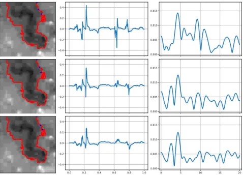
dashed rectangle. . . 24 4.1 The three selected images of capillary taken by a microscope. . . 26 4.2 The evolution of the given curve (red) on the given three different images

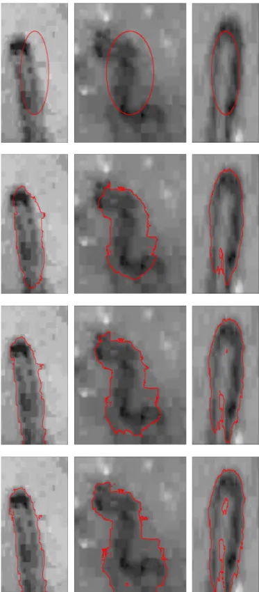
to detect the edge of the capillary. From top to below images show the iteration: 0, 20, 70, 150 except the lowest middle image which is the result of iteration 10,000. This image needs more iteration since the curve keep evolving at iteration 150. . . 28 4.3 The red curve (first column) is the outer edge of the capillary while the

blue star is the first three points to calculate the curvature. From upper to below, the distance of these points is longer. The middle and the third column shows the curvature and the magnitude of the Fourier transfor- mation. . . 29 4.4 The red curve (first column) is the outer edge of the capillary while the

blue star is the first three points to calculate the curvature. From upper to below, the distance of these points is longer. The middle and the third column shows the curvature and the magnitude of the Fourier transfor- mation. . . 29 4.5 The red curve (first column) is the outer edge of the capillary while the

blue star is the first three points to calculate the curvature. From upper to below, the distance of these points is longer. The middle and the third column shows the curvature and the magnitude of the Fourier transfor- mation. . . 30

vi

List of Figures vii 4.6 The red curve (first column) is the outer edge of the capillary while the

blue star is the first three points to calculate the curvature. From upper to below, the distance of these points is longer. The middle and the third column shows the curvature and the magnitude of the Fourier transfor- mation. . . 31 4.7 The red curve (first column) is the outer edge of the capillary while the

blue star is the first three points to calculate the curvature. From upper to below, the distance of these points is longer. The middle and the third column shows the curvature and the magnitude of the Fourier transfor- mation. . . 31 4.8 The red curve (first column) is the outer edge of the capillary while the

blue star is the first three points to calculate the curvature. From upper to below, the distance of these points is longer. The middle and the third column shows the curvature and the magnitude of the Fourier transfor- mation. . . 32 4.9 The red curve (first column) is the outer edge of the capillary while the

blue star is the first three points to calculate the curvature. From upper to below, the distance of these points is longer. The middle and the third column shows the curvature and the magnitude of the Fourier transfor- mation. . . 32 4.10 All of the hand-drawn images are in 3 blocks: Training, Validation, and

Test. The first row of each block is labeled by straight while the second row of each block is wiggly. . . 34 4.11 The result of the process of the updating parameters of the first CNN

model. . . 34 4.12 Some images in the test dataset. The incorrect classification is shown in

the second row while the correct classification is shown in the first row. . 35 4.13 The results of the first CNN model when it is applied to the images of

capillary taken by a microscope. . . 35 4.14 The result of the process of the updating parameters of the model. . . 36 4.1 The accuracy and loss of each category from the second CNN model. . . . 37 4.15 The results of the second CNN model applied to the images of capillary

taken by a microscope. The score in each category is presented by the

horizontal bar next to each image. . . 38

Chapter 1

Introduction

The content of this chapter describes a brief explanation of the image. For detail obser- vation, the image of the capillaries is chosen as the main topic discussion.

1.1 Image

One of the main topic discussions of this research is a digital image. An image is the visualization of an object. It is the output of some devices, for example, cameras, microscopes, etc. Those devices see images as the collection of numbers which can be a matrix of two or three dimensions. The most appropriate way to see the image is as a function.

Let f : Ω ⊂ R

→ R

where Ω is open, bounded, and rectangular domain, n ∈ N.

If n = 1, it is called a monochrome, a grayscale, or a brightness image. If n = 3, then it is a color image. The most well-known color image is an RGB image. RGB is the abbreviation of red green and blue which forms the basis for the other colors. An example of this RGB image and their decomposition is shown in the right and the left of Figure 1.1 respectively. The color image is the main focus on chapter 3, while chapter 2 focuses on the brightness image.

One categorizes an image to be static or dynamic. The static image does not change with respect to the time. Otherwise, it is a dynamic image. The dynamic image is well-known as a video. The image in this study refers to the static image.

Numbers f (x), where x ∈ Ω, is called a pixel value. If the image is monochrome, then the pixel values represent the brightness level. This pixel value is a nonzero integer up to 2

− 1 for some m ∈ N. When m = 1, it is well-known as the black and white image

1

Chapter One 2

red channel

blue channel

Figure 1.1: The left image is (256× 512) -color image taken by a camera in the festival of Hyakumangoku at Kanazawa, 2019. Its decomposition with respect to the red, green,

and blue channel are shown in the right.

or binary image. If m is higher, then the pixel values lie in the wider range. In this study, the range value of the images is [0, 255].

Images are important and interesting objects of study. There are some challenging problems involving the image, for example, image classification, segmentation, recon- struction, recognition, etc. It has been widely applied to many fields such as medical, robotics, informatics, etc. The focus of this study is image classification.

This study focuses on the brightness images for the PDE approach and the color images for the CNN approach. Hence, we can use the simple method to convert the color images into the brightness images, for example, linear combination. On the other hand, we can copy the pixel values of the brightness images to get RGB format images.

1.2 Capillaries

Capillaries are the smallest-diameter blood vessels which connect arteries to veins. The

size of capillaries is about 5 to 10 micrometers in diameter and their diameter averages

Chapter One 3

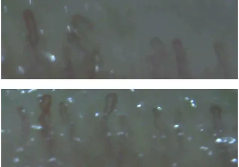
Figure 1.2: The image of capillaries taken by a microscope. The upper and below images are taken from different fingertips.

8 micrometers [6]. According to a private discussion with medical experts, there is a medical research that suggests that the shape and other features of human capillaries are linked to other health measures. Ogawa [14] outlined that the health of a person affects the shape of capillaries at the root of a fingernail. [20] also reported that the structure of capillaries is strongly related to serious diseases: connective tissue disease, diabetic Mellitus, and cancer. Hence, in the preventive medicine field, examining the capillaries status is important as a diagnostic tool.

In general, checking capillaries directly is not easy, for example, when examining the capillaries at eye’s fundus, the dilation of the pupil is required. However, by assuming the capillary is the track of the red blood cells, then capturing the image of the capil- laries around the root part of a fingernail can be conducted just by a microscope with magnification around 700-900. Thus, it is possible even to conduct the observation with a cheap microscope and record the changes of the patterns easily. Figure 1.2 show exam- ples of capillaries on human fingertips taken by 700-900 magnification of a microscope.

The lens of the microscope were located on the skin near the root of a fingernail.

However, diagnosis based on these images is not an easy task because it requires the

skill of medical experts (doctors). This skill is unique and not every doctor can perform

this diagnosis. Different doctors might give different diagnosis results. Hence, by the

motivation of how to learn the diagnosis from the skilled medical experts and how to

develop a consistent diagnosis, the problem is how to learn the structure of capillaries

from its image.

Chapter One 4

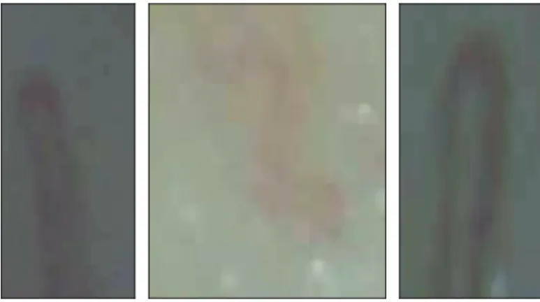
Figure 1.3: The images of artificial capillaries for the straight (left) and wiggly (right).

The starting point of this paper is the research work by Hung, Nakane, and Hashimoto [9] which developed a judgment category by measuring curve oscillation. They presented the images of capillaries for both healthy and unhealthy persons. According to those images, the straight capillary is related to healthy persons, while the wiggly capillary is related to unhealthy persons. The straight capillary has a shape expressed by a U-configuration. Let consider this U-shape as a turning point. We said the straight capillary has at most one turning point. However, if the shape of capillary has at least two turning points, then the capillary is wiggly.

The purpose of this research is to judge the status of images by (i) PDE approach and (ii) CNN approach according to medical motivation. The output of the first approach is either straight or wiggly, but the more details explanation cannot be added. For the second approach, the output is not only straight or wiggly but also several abnormal patterns of the capillaries.

The base of the PDE approach is the active contour method to detect the edge of an object in the brightness image input. The curvature is then estimated along the edge.

The curvature is analyzed using the Fourier transform. The output is the frequency that corresponds to the peak magnitude. If such frequency is zero, then the status image of the input is straight. If such frequency is nonzero, then the status image of the input is wiggly. Unfortunately, the abnormal patterns of the capillaries are classified as the wiggly by this PDE approach. Thus, we present the second approach, that is CNN.

We report two models of the CNN approach. The first model of CNN has two categories

that are straight and wiggly. We use the images of artificial capillaries to train the

CNN model. These images are created by hand and labeled intentionally based on

the images of real capillaries in [3] for each straight and wiggly, as shown in Figure

1.3. Actually, the wiggly capillary has a meaningless meander which is a complicated

structure. Unfortunately, the meaning of these complicated structures is very difficult

to transfer the information or technique to other doctors.

Chapter One 5 The first model of CNN can distinguish the structure of capillaries into two rough cate- gories, but no further information can be added by this model. We think it is insufficient because (i) skill cannot be transferred to other doctors, (ii) the causes and the effects are not clear, which is not good for further research, and (iii) new detail explanation cannot be found. To overcome these problems, we divide the meaning of the complicated structures into several patterns such as wiggly (meaningless meandering), unexpected separation pattern, a vague edge which the blood exudes on the random part of cap- illaries, and branch appearing. The edge is the boundary of an object on the image.

Therefore, the second model of CNN has nine categories, that are straight fine, straight 1 branch, straight 2 branches, straight jump, straight sharp, wiggly fine, wiggly 1 branch, and wiggly 2 branches, wiggly jump. The first category is the simple structure without any abnormal type. The second category is the simple structure with a branch point.

The third category is the simple structure with two branches points. The fourth cate- gory is the simple structure with a jump. The fifth category is the simple structure with sharp oscillation. The sixth category is the meandering pattern without any separation and branch. The seventh to ninth category is similar to the second to fourth category respectively except the pattern which is meandering type.

This model also uses the image of artificial images for each category. Instead of jumping directly into nine categories as the second CNN model, we report the first CNN model to assure that the CNN approach can work well as the first approach.

Here is the brief summary of our strategy of the second CNN approach:

1. Segmentation of notions.

We divide the abnormal types of capillaries into several patterns such as meander- ing, unexpected separation pattern, and branch appearing.

2. Defining a mathematical category for each pattern.

We give a stage number for each pattern. Here is the example: (i) by using the image processing which is PDE approach, we give meandering category for the case meaningless meandering, (ii) we count the number of ^‘ separation ^’ or ^‘ branch ^’ points and give indicator, and (iii) for the case of vague edge, we give indicator by measuring the vague part ratio by naked eye or image processing.

3. Creating artificial data for training. We create training image data with indicators for each pattern.

4. Train CNN using artificial data.

Generally, CNN requires a large number of images in training data. All these images

determine the adjusted parameters during training. However, this can be tackled by the

Chapter Two 6

transfer learning that leads to a reduction in the number of trainable parameters. The

transfer learning means we copy the model and its optimum parameters. This model

is a so-called pre-trained. We select VGG16 as the pre-trained model in this study

and combine it with our network. Hence, the input of the images is feeding up to the

pre-trained model first, and then the output becomes the input to our network. As a

consequence, the number of images used in training can be much declined. Besides, the

patterns of the capillaries are not as much complex as image classification between cats

and dogs. Hence, the number of image data is still able to be decreased. The benefit

of this approach is the possibility to train CNN by a small number of test data. The

other merit is not only the capillaries are classified into straight and wiggly, but the

damage of capillaries is also classified. The output is expressed by numbers (score) for

each category. This score means how close the input image to the training data of each

category.

Chapter 2

Partial Differential Equation

Approach on Edge Detection and Its Classification

The given image in this chapter is limited to the monochrome or brightness image. We propose the PDE approach to judge the image. The summary of this approach is given in Figure 2.1. The output of this approach is that the given input image is either straight or wiggly. From these outputs, we cannot add detail information about the abnormal pattern of capillaries. The first is a method to detect the edge of an object on a given image. The curvature of a given curve is the second. The last is the Fourier transform of a given function.

2.1 Edge Detection

Let f : Ω → R be a given image, where Ω ⊂ R

is an open and bounded set. Assume that there is at least one object drawn on the given image f. This is called an object when it has a different brightness value than the background. The edge of this object refers to the location where there is a discontinuity on f . Mathematically, E ⊂ Ω is the edge if and only if f (x, y) is discontinuous for every (x, y) ∈ E. Hence, the mathematical problem of edge detection is how to find E from the given image f .

2.1.1 Gradient method

Looking at the gradient of f might be the first attempt since it is quite simple and fast.

The edge of an object on image f is E = { (x, y) ∈ Ω | |∇f (x, y)| 6= 0 } . However, it

7

Chapter Two 8

Input the brightness image

Detect the edge of the object by the ac- tive contour method

The curve of the edge of the object Estimate the curva-

ture of the curve

The approximated curveture along

the curve

Fourier transform

The magnitude that corresponds to the frequency kp: The frequency

at which the peak magnitude occurs

Ifkp= 0, then the input image is

straight

Ifkp6= 0, then

the input image is wiggly

Figure 2.1: The summary of the PDE approach to judge the image.

Chapter Two 9 is quite problematic if there exists a noise on f . Generally, these happen very often.

As a consequence, it gives an unwanted result E which now contains the edge and the location of the noise. Therefore, another approach is needed to get E containing exactly the edge. One of them is the optimization approach.

There have been several different methods when the optimization approach is selected, for example, Split Bregman [8], Perona-Malik [15], Mumford-Shah [3], or Canny method.

This study selects the active contour method since it is quite relevant to the specific image of capillary later.

2.1.2 Active contour method

For more details, please see [4]. The active contour method is a segmentation between object and background in the image. The object indicates the different brightness value with the background.

2.1.2.1 Basic formulation

Let f : Ω → R be given where we assume the object exists in f . The open subset ω ⊂ Ω is related to the object in Ω and the background is related to Ω\ω. Then we define the functionals as follows:

F

(ω, c

, c

) = λ

Z

ω

|f (x) − c

|

dx + λ

Z

Ω\ω

|f (x) − c

|

dx + γ|∂ω| (2.1)

where c

and c

are constant, |∂ω| is the length of the boundary of ω, and λ

, λ

, γ > 0

are fixed parameters. Minimizing the first two terms in the right-hand side (RHS) of

(2.1) means that the curve will coincide to the edge of an object on f. While minimizing

the last term in RHS of (2.1) means we want the curve as shortest as possible. Finally,

minimizing the functional F

means finding ω which its boundary is as shortest as

possible and coincides to the edge of an object on f . Taking the first variation of F

is

complicated so that we need to express F

in the other way by level-set formulation.

Chapter Two 10 2.1.2.2 Level-set formulation

Let φ : Ω → R be a Lipschitz function such that

∂ω = {(x, y)|φ(x, y) = 0}

ω = {(x, y)|φ(x, y) > 0}

Ω\ω = {(x, y)|φ(x, y) < 0}.

We approximate the Heaviside and the delta Dirac function in the distributive sense by smooth functions as follows:

H

(x) = 1 2

1 + 2

π arctan x

and

δ (x) = dH (x)

dx =

π (

+ x

) .

Thus, we introduce a functional F

related to F

as the following, F

(φ, c

, c

) = λ

Z

Ω

|f (x) − c

|

H (φ)dx + λ

Z

Ω

|f (x) − c

|

(1 − H (φ))dx

+ γ Z

Ω

δ (φ)|∇φ|dx. (2.2)

F

is an approximation of F

.

Let fix φ and c

. We define one-dimensional real function, G

(c

) := F

(φ, c

, c

).

The derivative is

dG

dc

= 2λ

Z

Ω

(f (x) − c

)H (φ)dx.

We obtain

= 0 if

c

= R

Ω

f (x)H

(φ)dx R

Ω

H (φ)dx . (2.3)

The denominator is not zero if |ω| 6= 0.

Let fix φ and c

. We define one-dimensional real function,

G

(c

) := F

(φ, c

, c

).

Chapter Two 11 The derivative is

dG

dc

= 2λ

Z

Ω

(f (x) − c

) (1 − H

(φ)) dx.

We obtain

1

= 0 if

c

= R

Ω

f (x) (1 − H

(φ)) dx R

Ω

(1 − H (φ)) dx . (2.4)

The denominator is not zero if |Ω\ω| 6= 0.

The minimizer of c

and c

obtains from (2.3) and (2.4) respectively. From this formula, when we know φ, then c

and c

can be calculated directly. This means we can write F

(φ) instead of F

(φ, c

, c

).

The remained variable that needs to be considered is φ. Let Φ ∈ C

(Ω, R), the first two terms of F

is F

, and the last term of F

is F

. By taking the first variation of F

with respect to φ, we get

d

dν F

(φ + νΦ)

= d dν

λ

Z

Ω

|f (x) − c

|

H (φ + νΦ) dx

+λ

Z

Ω

|f (x) − c

|

(1 − H (φ + νΦ)) dx

= λ

Z

Ω

|f (x) − c

|

δ

(φ) Φdx − λ

Z

Ω

|f(x) − c

|

δ

(φ) Φ dx.

By taking the first variation of F

with respect to φ, we get d

dν F

(φ + ν Φ)

= d dν

γ

Z

Ω

δ (φ + νΦ)|∇φ + νΦ| dx

= γ Z

Ω

d

dν (δ (φ + νΦ) |∇φ + ν∇Φ|)

dx

= γ Z

Ω

δ (φ) d

dν |∇φ + ν∇Φ|

+ |∇φ + ν∇Φ| d

dν δ (φ + νΦ)

dx

= γ Z

Ω

δ (φ) ∇φ · ∇Φ

|∇φ| + |∇φ|Φδ

(φ) dx

= γ Z

Ω

− div

δ (φ) ∇φ

|∇φ|

Φ + |∇φ|Φδ

(φ) dx

= γ Z

Ω

−δ

(φ) div ∇φ

|∇φ|

Φ − ∇ (δ (φ)) · ∇φ

|∇φ|

Φ + |∇φ|Φδ

(φ) dx

= γ Z

Ω

−δ

(φ) div ∇φ

|∇φ|

Φ − δ

(φ) ∇φ · ∇φ

|∇φ|

Φ + |∇φ|Φδ

(φ) dx

= γ Z

Ω

−δ

(φ) div ∇φ

|∇φ|

Φ − δ

(φ) |∇φ|Φ + |∇φ|Φδ

(φ) dx

= γ Z

Ω

−δ

(φ) div

∇φ

|∇φ|

Φ dx.

Chapter Two 12 Therefore, we get,

d

dν F

(φ + ν Φ)

= d

dν F

(φ + ν Φ)

+ d

dν F

(φ + νΦ)

= λ

Z

Ω

|f(x) − c

|

δ

(φ) Φdx − λ

Z

Ω

|f (x) − c

|

δ

(φ) Φ dx

− γ Z

Ω

δ (φ) div

∇φ

|∇φ|

Φ dx.

2.1.2.3 Gradient descent method

In this subsection, we consider the time-dependent problem, φ : [0, ∞) × Ω → R. Taking the first variation of F

in (2.2) with respect to φ and applying the gradient descent method lead to,

∂φ

∂t = δ

(φ)

−λ

|f − c

|

+ λ

|f − c

|

+ γdiv ∇φ

|∇φ|

in (0, ∞) × Ω, (2.5a)

φ = φ

in {0} × Ω, (2.5b)

∂φ

∂n = 0 on (0, ∞) × ∂Ω. (2.5c)

where φ

: Ω → R and

denotes normal derivative of φ at the boundary.

Let φ

be the solution of (2.5). Then the edge of an object on f is the curve C

, the zero level set of φ

. We stop the iteration when the zero level set of {φ

} converge because the main concern is the zero level set. Finite difference method is used to find the approximation of the solution of (2.5). The algorithm 1 shows the detailed implementation. All the given images when we apply this method in fourth chapter have m

and m

not greater than 280.

2.2 Estimation of Curvature

We show a brief explanation about curvature here. For more details, see [7]. Let ζ(s) = (x(s), y(s)) where s ∈ [0, 1] be the parametric representation of ∂ω, where x, y : [0, 1] → R, both x and y are twice continuously differentiable, and |ζ

| 6= 0. Let T

(s), N

(s), and k

(s) be a unit tangent vector, unit normal vector, and the signed curvature respectively of the curve ζ at s. Note that k

: (0, 1) → R. Hence,

T

(s) = 1

|ζ

(s)| x

(s), y

(s)

Chapter Two 13

Algorithm 1 Finding the solution of (2.5) Given:

f

is the image where i = 0, 1, . . . , m

− 1, j = 0, 1, . . . , m

− 1 H

(x) =

1 +

arctan

δ

(x) =

Choose:

λ

= λ

= 1, γ = 10, = 0.01: Fix the parameters h

= 10

: Time step

h

=

1−1

, h

=

2−1

: Space step Calculate:

φ

: [0, 1] × [0, 1] → R φ

= 3 −

r

m₁−1

−

+ 2

j

m₂−1

−

(Initial function) C

← The zero level set of φ

(Make sure |C

| 6= 0)

c

←

Pm1−1 i=0

Pm2−1 j=0 f_ijH

φ⁽⁰⁾_ij Pm1−1

i=0

Pm2−1 j=0 H

φ⁽⁰⁾_ij

c

←

Pm1−1 i=0

Pm2−1 j=0

1−H

φ⁽⁰⁾_ij

fij

Pm1−1 i=0

Pm2−1 j=0

1−H

φ⁽⁰⁾_ij

n ← 0 (Initial timestep) while C

not converged do

n ← n + 1

φ

← Apply finite difference method in the Equation (2.5a) and (2.5c) C

← The zero level set of φ

c

←

Pm1−1 i=0

Pm2−1 j=0 fijH

φ⁽ⁿ⁾_ij

Pm1−1

i=0

Pm2−1 j=0 H

φ⁽ⁿ⁾_ij

c

←

Pm1−1 i=0

Pm2−1 j=0

1−H

φ⁽ⁿ⁾_ij

f_ij Pm1−1

i=0

Pm2−1 j=0

1−H

φ⁽ⁿ⁾_ij

end while Result:

C

and

N

(s) = 1

|ζ

(s)| y

(s), −x

(s)

where s ∈ (0, 1). Curvature is one of the tools to measure how much the curve bends from its tangent line. The curvature of a curve which is straight line is zero. It can be formulated as

k(s)N (s) = lim

h→0

T

(s + h) − T

(s) h

= 1

|ζ

(s)|

x

(s)(y

(s))

− y

(s)y

(s)x

(s) , y

(s)(x

(s))

− x

(s)x

(s)y

(s)

.

Chapter Two 14 Therefore,

k(s) = x

(s)y

(s) − y

(s)x

(s)

|ζ

(s)|

, (2.6)

where s ∈ (0, 1). Finite difference method is used to approximate the curvature in (2.6).

2.3 Analysis Using Fourier Transform

For more details explanation, see [1]. Let η : R → R, then the Fourier Transformation of η, denoted by η, is defined by ˆ

ˆ η(k) =

Z

−∞

η(x)e

dx. (2.7)

Note here that η ˆ : R → C. Let k be so-called the frequency. Let call |ˆ η(k)| the magnitude at the frequency k. This magnitude is an even function. Therefore, we consider the nonnegative k in this research.

One might notice that if η is defined on the domain [0, 1], then η ˆ is calculated by

ˆ η(k) =

Z

η(x)e

dx. (2.8)

This give a similar result to when we set η = 0 outside (0, 1) and calculating 2.7. Since (2.8 ) is used later, then we focus on this case.

Theorem 2.1. Let η : [0, 1] → R, if 0 < η(t), ∀t ∈ [0, 1], then the peak magnitude occurs at zero frequency.

Proof. Since η is a positive function, then

|ˆ η(k)| =

Z

η(x)e

dx

≤ Z

0

η(x)e

dx =

Z

|η(x)| dx = Z

0

η(x) dx

for every k . While for k = 0 , we have

|ˆ η(0)| =

Z

η(x) dx

= Z

0

η(x) dx.

The last equality holds since η is a positive function. Therefore, the peak magnitude occurs at zero frequency.

Corollary 2.2. If η(t) < 0, ∀t ∈ [0, 1], then the peak magnitude also occurs at zero

frequency.

Chapter Two 15 Here are the relevant basic properties:

1. Linearity

Let η

, η

, η

: [0, 1] → R and η

= η

+ η

, then

ˆ η

(k) =

Z

η

(x)e

dx

= Z

0

(η

(x) + η

(x)) e

dx

= Z

0

η

(x)e

dx + Z

0

η

(x)e

dx

= ˆ η

(k) + ˆ η

(k).

2. Translation

Let η

, η

: R → R and η

(x) = η

(x − c) for some c ∈ R, then ˆ

η

(k) = Z

−∞

η

(x)e

dx

= Z

−∞

η

(x − c)e

dx

= Z

−∞

η

(x − c)e

dx

= e

Z

−∞

η

(y)e

dy

= e

η ˆ

(k).

Moreover, |ˆ η

(k)| = |ˆ η

(k)| for every k . This means the magnitude of the frequency k for the Fourier transformation’s result of a function and its translation is the same.

We propose the analysis using Fourier transform since the curvature of the straight capillary can be considered as a Gaussian function based on the results in the last chapter. As a consequence, the peak magnitude occurs at the zero frequency. If the curvature oscillates significantly, then this curvature looks like a sine or cosine function for some nonzero frequency. Consequently, the peak magnitude will occur at the nonzero frequency. This is an interesting fact that gives much help in this study.

Let G

: R → R where G

(x) = ae

be the Gaussian function which has the

peak a at x = 0 ∈ I and has the slimness factor by b, where a, b ∈ R and b > 0. Let

Chapter Three 16

g(x) = G

(x) almost everywhere. Then ˆ

g(k) = Z

−∞

g(x)e

dx

= Z

−∞

ae

e

dx

= a Z

−∞

e

dx

= ae

2k2 b

Z

−∞

e

x+^πik_b

2

dx

= a √

√ π b e

2k2 b

.

This means the Fourier Transformation’s result of a Gaussian function is also Gaussian function with different peak value and slimness factor.

Let G be any Gaussian function, from second and third properties then G ˆ is a Gaussian

function which might have different peak value and slimness factor than G , but the peak

value of the magnitude always occurs at the zero frequency.

Chapter 3

Convolutional Neural Network Approach

We propose the CNN approach to judge the status of the images according to medical motivation. We base our model on a pre-trained VGG16 model for the lower layers of the network and our implementation uses Python and the Torch library. Neural networks are first explained in this chapter since it is the basis of CNN. Then the details of the CNN are briefly described. The next is the explanation about the transfer learning. The last is our proposed model.

The CNN becomes exponentially quite popular in these recent years. It is the most powerful tool used for a large-scale image recognition [12], [17], and [18]. It is also applied to other classification problems, for examples, in [13] and [19]. In addition, it is applied to medical images [10], [5], [16], and [21]. For this reason, it is chosen as an important approach in this study. This chapter explains briefly about CNN, for more details, see [2].

3.1 Neural Networks

Mathematically, one describes a neural network as a mapping from a set of inputs to a set of outputs which is determined by the parameters that can be adjusted. This mapping can be a composition of two or more functions. There are many possibilities of how the setting of this composition, what kind of functions, or how many parameters needed. The explanation in this section does not cover all of them, but we give one example to get a better understanding of the neural networks.

17

Chapter Three 18

Input

Layer-1

.. .

Layer-2

.. .

. . . Layer-n

.. .

. . . Layer-N

.. .

Ouput

Figure 3.1: A sample of N -layers neural networks. The circle or node indicates the perceptron.

There is another way to interpret a neural network. One can see it as the process of a set of inputs that pass through one or more layers, where there is a set of nodes in each layer, before producing a set of outputs. One might say the second layer up to N − 1 is the hidden layer. One sometimes might say the node as the perceptron. Figure 3.1 shows an example of a model of a fully connected neural network with N -layers. A neural network does not need to be always fully connected.

For more details, let an input, the number of layers, and the number of nodes in layer- n be given by {x

∈ R | i = 1, 2, 3, . . . , M } , N , and Q

∈ Z

respectively where n = 1, 2, 3, . . . , N. The model is fully connected as in Figure 3.1. The output of node-q at first layer, indicated by the superscript (1), is then

y

= f





M

X

p=1

w

x

+ w



 , (3.1)

where q = 1, 2, 3, . . . , Q

, f

: R → R is a nonlinear function called the activation,

and w

∈ R for p = 1, 2, 3, . . . , M is the parameter called by the weight and w

∈ R

is the parameter called by the bias ∀q = 1, 2, 3, . . . , Q

. For the activation function

f : R → R, there exists several choices. Here are some examples, f (x) = tanh(x),

f (x) = 1/ (1 + exp(−x)), f (x) = max(x, 0), and etc. The idea is how to get the output

numbers between 0 and 1 or a positive. It is motivated first by the output is between

Chapter Three 19 yes or no which means 0 or 1, but it is extended to be a real number between 0 and 1 or even be positive real numbers.

Next, the set of input for the next layer is the set of the output from the previous layer.

At layer-n, the output of node-q is

y

= f





Q⁽ⁿ⁻¹⁾

X

p=1

w

y

+ w



 , (3.2)

where n = 2, 3, 4, . . . , N, q = 1, 2, 3, . . . , Q

, f

: R → R is the activation function, and w

∈ R is the weight and w

∈ R is the bias for every p = 1, 2, 3, . . . , Q

, q = 1, 2, 3, . . . , Q

and n = 2, 3, 4, . . . , N .

From those examples, it can be deduced in the simple and very general way that a neural network is a mapping

F ( x , w ) = y

where x is the set of inputs, w is the set of all parameters, and y is the set of outputs that correspond to the input. In practice, how to set the mathematical problem depends on the specific purpose. For example, one can set the number of layers, the number of nodes in each layer, the activation function, fully connected or not, and the targeted output, this will be explained later. Then the mathematical problem is how to choose the parameters w such that the given input x maps correctly into the target output.

3.1.1 Loss function

The loss function is used to measure how close the output to the targeted output. The targeted output means the desired output which is independent of w. If it is given or it is labeled first, then the training, it will be explained later, is called supervised.

Otherwise, it is unsupervised. Sometimes it is well-known as the errors function.

Let T = t

∈ R

| M

∈ Z

, i = 1, 2, 3, . . . , M

∈ Z

be the given set of the targeted output. This set is required to be linearly independent. M

indicates the number of categories. For the example as in Figure 3.1, then M

= Q

. The simplest way for the choice of the targeted output is by setting M

= M

and i -th entry of t

is 1 and the others are 0.

Let t

∈ T be the corresponding targeted output of the given input x

. One chooses the loss function as the following,

E =

N0

X

i=1

|F (x

, w) − t

|

(3.3)

Chapter Three 20 where N

is the given number of inputs. There is also another way to define loss function than (3.3).

After defining the loss function, the problem is then how to find the parameters w which are able to minimize the given loss function. As a consequence, one can use the gradient descent method. The process of how to find the minimizer is called training or learning.

3.2 Convolutional Neural Networks

Actually, that model can be interpreted as extracting quite details information from each component of the input. This input can be the pixel of the image, the audio, or the others. For the image classification or recognition, it does not need to extract very details information from each pixel. There can be some pixels which do not give the desire or important information, for example, the background. There can also be the noise of the image. Hence, it is needed to extract information from the local area, a small sub-region of the image. It is also needed, if possible, to be able to deal with the translation, small rotation, and dilatation. In addition, the most important is how to extract the features of the given image. Hence, all of these can be handled by the CNN, where its ideas are local receptive area, the sharing weight, and sub-sampling.

Here are some advantages when applying a CNN. First, the local receptive area keeps the spatial domain of the input. Second, the sharing weight affects the number of parameters is much reduced. Third, whenever the input image is translated, the activations of the feature map are translated by the same amount, but the other feature maps are not changed.

For the calculation, those first two ideas affect that the convolution is needed, instead of component-wise multiplication. For example, let the input be x = ((x

)) ∈ M

, an image of the size (m

, m

), and the activation function f

be defined component-wise.

For example, if z = ((z

)) ∈ M

, then f

(z) = ((f (z

))) ∈ M

where f : R → R. The output of node-q at first layer, indicated by the superscript (1), is

y

= f

w

∗ x + w

, (3.4)

where q = 1, 2, 3, . . . , Q

, the output y

∈ M

(1)

1 ×q₂⁽¹⁾

for some q

≤ m

, q

≤ m

, the weight or known by the kernel is w

∈ M

(1) q1×m⁽¹⁾_q

2

, the bias is w

∈ M

(1) 1 ×q₂⁽¹⁾

, and the component-wise activation is f

. For the layer-n, the output of node-q is

y

= f





Q⁽ⁿ⁻¹⁾

X

p=1

w

∗ y

+ w



 , (3.5)

Chapter Three 21 where n = 2, 3, 4, . . . , N , q = 1, 2, 3, . . . , Q

, the output y

∈ M

(n)

1 ×q⁽ⁿ⁾₂

for some q

≤ q

, q

≤ q

, the weight or known by the kernel is w

∈ M

(n) q1 ×m⁽ⁿ⁾q2

, the bias is w

∈ M

(n)

1 ×q₂⁽ⁿ⁾

, and the component-wise activation is f

.

The last is sub-sampling. There are several ways to calculate the sub-sampling, for example, by using the average of the local area or the maximum value of the local area.

If this local area is chosen to be (2 × 2)-size, then the size of the output of the sub- sampling is reduced around a half. Actually, the local area can be chosen to be another size.

One should notice that for CNN, it is typical that the final layer is a fully connected layer. Perhaps some layers before the final layer are already a fully connected layer. The input for this layer is flattened first, then (3.2) is used. This happens since the output does not need to be spatially maintained.

3.3 Transfer Learning

Building or creating the optimum model is not an easy task. There are too many possibilities that can be selected, for example, how many layers needed, the size or number of the kernel that appropriates in each layer, etc. Even if we have already chosen a model, there is a high possibility that the number of images in training dataset is not enough to get the optimum parameters during training. This is because too many parameters that need to be obtained. Therefore, transfer learning is a suitable alternative way.

Transfer learning means that the model and its optimum parameters after being trained by the others on a huge amount of training dataset is being transferred or copied. That model is a so-called pre-trained model. More layers are added at the end of that model.

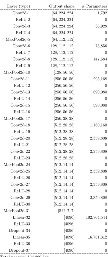
Now, the number of parameters can be reduced so much. As a consequence, the number of images on the training dataset can be reduced too. An example of that pre-trained model, which is chosen in this research, is VGG16. We use the first 37 layers of this pre-trained model, as shown in Table 3.2. The output of this pre-trained model becomes the input of our proposed model.

VGG is the abbreviation for Visual Geometry Group. This VGG16 model was devel-

oped by Si- monyan and Zisserman from Department of Engineering Science, University

of Oxford. It is a very deep CNN model. It was the basis of their ImageNet Challenge

2014 submission, where their team secured the first and second places in the localization

and classification tracks respectively [18]. VGG16 classifies images into 1000 categories.

Chapter Three 22 Among these categories, some examples are snakes, spoons, microphones, and paint- brushes. We assume the complicated structures of capillaries are similar to snakes and the simple structures are similar to spoons, microphones, or paintbrushes. The input images of VGG16-model are in RGB format of fixed 224 × 224-size. We use the first 37 layers of this pre-trained model, as shown in Table 3.2. The output of this pre-trained model becomes the input of our proposed model.

3.4 The Proposed Model

We propose a model of a fully connected layer consisting of 5 layers. The first layer consists of 256 nodes. Consequently, this layer requires 1,048,832 parameters because the output from the pre-trained model has 4,096 nodes. Let the output of the pre-trained model be y

∈ R

. Thus, the output of layer p

is

y

= w

y

+ w

where y

, w

∈ R

and w

∈ M

. The output of layer p

is y

= max

y

, 0

where i = 1, 2, . . . , 256. The Dropout in layer p

has factor 0.2 which means 20% of the output of this layer in each channel is deactivated randomly. The output of layer p

is

y

=







y

if node-i is activated 0 if node-i is deactivated where i = 1, 2, . . . , 256. Layer p

have the output as follows,

y

= w

y

+ w

where y

∈ R

is the output of layer p

, y

, w

∈ R

and w

∈ M

for the number of categories, n.

The last layer is LogSoftmax, an activation function, where the output of this layer p

is

y

= log





exp y

P

j=1

exp y





for i = 1, 2, . . . , n. We propose two CNN models. The first model is of n = 2 and the

second model is of n = 9 . The summary of the second approach is given in Figure 3.3.

Chapter Three 23

Figure 3.2: The first 37 layers of the model of VGG16.

Layer (type) Output shape # Parameters

Conv2d-1 [64, 224, 224] 1,792

ReLU-2 [64, 224, 224] 0

Conv2d-3 [64, 224, 224] 36,928

ReLU-4 [64, 224, 224] 0

MaxPool2d-5 [64, 112, 112] 0

Conv2d-6 [128, 112, 112] 73,856

ReLU-7 [128, 112, 112] 0

Conv2d-8 [128, 112, 112] 147,584

ReLU-9 [128, 112, 112] 0

MaxPool2d-10 [128, 56, 56] 0

Conv2d-11 [256, 56, 56] 295,168

ReLU-12 [256, 56, 56] 0

Conv2d-13 [256, 56, 56] 590,080

ReLU-14 [256, 56, 56] 0

Conv2d-15 [256, 56, 56] 590,080

ReLU-16 [256, 56, 56] 0

MaxPool2d-17 [256, 28, 28] 0

Conv2d-18 [512, 28, 28] 1,180,160

ReLU-19 [512, 28, 28] 0

Conv2d-20 [512, 28, 28] 2,359,808

ReLU-21 [512, 28, 28] 0

Conv2d-22 [512, 28, 28] 2,359,808

ReLU-23 [512, 28, 28] 0

MaxPool2d-24 [512, 14, 14] 0

Conv2d-25 [512, 14, 14] 2,359,808

ReLU-26 [512, 14, 14] 0

Conv2d-27 [512, 14, 14] 2,359,808

ReLU-28 [512, 14, 14] 0

Conv2d-29 [512, 14, 14] 2,359,808

ReLU-30 [512, 14, 14] 0

MaxPool2d-31 [512, 7, 7] 0

Linear-32 [4096] 102,764,544

ReLU-33 [4096] 0

Dropout-34 [4096] 0

Linear-35 [4096] 16,781,312

ReLU-36 [4096] 0

Dropout-37 [4096] 0

Total params: 134,260,544 Trainable params: 0

Non-trainable params: 134,260,544

1

Chapter Three 24

Input the color image VGG16

output-4096 ... output-6 output-5 output-4 output-3 output-2 output-1

Layer-p1

...

Layer-p2

...

Layer-p3

...

Layer-p4

...

Layer-p5

...

Ouput

Figure 3.3: The flow chart of the second approach. The proposed model is in the dashed rectangle.

The loss function that we choose in this research is the Average Negative Log Likelihood.

Since the final layer score is already the LogSoftmax-layer, then multiplying by negative one is enough. We define T as the set of targeted output. Let M ∈ Z

be the number of images in training, y

∈ R

be the output of the layer p

for m

-image, and t

∈ T be the targeted output of m

-image. Since the final layer is LogSoftmax, then the negative log-likelihood is defined as

L(y

, t, w, M ) = 1 M

M

X

m=1

−y

m

where y

is the set of the output of layer p

for all M images, t is the set of the targeted output for all M images, w is the set of trainable and non-trainable parameters.

For the first CNN model, the number of categories is two. Thus, the set of the targeted output is T = { (1, 0) , (0, 1) } where (1, 0) belongs to the first category and (0, 1) be- longs to the second category. The second CNN model has nine categories. Thus, the targeted output for the category-i is t

∈ R

where the i

-component is 1 and the other components are 0.

Adam method is implemented to find the minimizer of L with respect to the trainable parameters. This method computes individual adaptive learning rates for different pa- rameters from estimates of first and second moments of the gradients [11]. The name of this method is derived from the adaptive moment estimation.

The output of the CNN model is the score for each category. This score means how

close the input image to the training data of each category. Increasing the number of

training images might get better results. From this score, we determine that the input

image is classified to the highest score category. We also state that the image is classified

Chapter Four 25 correctly if the highest score category is the same as the label of that image. We define average accuracy by

m

M × 100%,

where m

is the number of images which classified correctly, and M is the number of

input images. Finally, all of the setup the CNN in this research is implemented in Python

and Torch.

Chapter 4

Application on the Image of the Capillaries

The main goal in this chapter is how to classify the capillary into two categories, that are straight and wiggly. There are two different approaches to this classification. First is the partial differential equation approach. The second is the convolutional neural network approach.

4.1 Partial Differential Equation Approach

We directly look at the image of the real capillaries. We provide three images as in Figure 4.1 to be evaluated by the partial differential equation approach. We decided and then labeled by our own naked eyes that the first and third cases are the straight capillary. The wiggly capillary is the second case.

Figure 4.1: The three selected images of capillary taken by a microscope.

26