A thesis submitted in fulfillment for the degree of Master of Finance

TOKYO METROPOLITAN UNIVERSITY

Regulatory Policy to Mitigate Potential Risks Arising from Contingent Convertibles

by

Hitomi Ito

A thesis submitted in fulfillment for the degree of Master of Finance

Department of Business Administration Graduate School of Social Sciences

January 2018

Abstract

A Contingent Convertible (CoCo) bond is an instrument that converts into equity or suffers a write-down when the issuing bank is in financial distress. In practice, a trigger event of CoCo takes place when the capital ratio of the bank falls to the pre-defined level or when the national authority declares a trigger at its discretion. The aims of this study are to model CoCos having such triggers and to find effective regulatory policies to handle them. A model for banks issuing CoCos is built within the framework of a structural-default approach. The trigger mechanisms are expressed in a first passage time model and in a stochastic intensity model. CoCo investors are also included in our model as CoCos are designed to enhance the bank’s resilience while shifting its risks to the investors. In the numerical example, we show that effective regulatory policy, which is intended to mitigate both banks’ and investors’ default risks, changes according to the correlation between banks and investors and the impact of the trigger event on the bank asset value process.

Keywords: Contingent convertible, structural approach, accounting trigger, regula-

tory trigger, systemic risk, regulatory policy

Acknowledgement

Foremost, I would like to express my deepest appreciation to my supervisor, Prof.

Masaaki Kijima of Master of Finance Program, Tokyo Metropolitan University. He has greatly supported and encouraged me throughout my research, while allowing me to proceed in my own way. Without his patience and knowledge, I would not have managed to improve my thesis to this extent. My appreciation also goes to professors in Master of Finance Program, Tokyo Metropolitan University, for supporting me around technical issues. I would also like to offer my special thanks to my classmates, Koji Anamizu and Eri Nakamura for contributing with insightful comments and suggestions.

Last but not least, I must appreciate my husband Shunsuke for his warm encouragement

throughout my study.

Contents

1 Introduction 1

1.1 Background . . . . 1

1.2 What is CoCo . . . . 2

1.2.1 Loss-Absorption Mechanism . . . . 3

1.2.2 Trigger Mechanism . . . . 3

1.3 CoCos in Real Markets . . . . 4

1.4 CoCos and Regulation . . . . 6

1.5 Literature . . . . 8

1.6 Aims of the Study . . . . 9

2 The Model Setup 10 2.1 Bank . . . . 11

2.1.1 General Framework . . . . 11

2.1.2 Type 0 Bank (Subordinated Bond) . . . . 14

2.1.3 Type 1 Bank (Equity-Conversion CoCo) . . . . 16

2.1.4 Type 2 Bank (Write-down CoCo) . . . . 18

2.2 CoCo Investor . . . . 20

2.3 Regulator . . . . 22

3 Numerical Example 24 3.1 Optimal Capital Structure . . . . 24

3.2 Default Probabilities . . . . 28

3.3 Regulatory Policy . . . . 32

4 Conclusion 35 4.1 Effective Regulatory Policy . . . . 35

4.2 Future Work . . . . 37

A First Passage Time 39

B Calculation of Firm Value 42

B.1 Discrete-Time Accounting Trigger . . . . 42

B.1.1 Proof of (B.7) . . . . 44

B.1.2 Proof of (B.8) . . . . 45

B.2 Regulatory Trigger Added . . . . 45

Chapter 1 Introduction

A Contingent Convertible (CoCo) is a new type of financial instrument that came along with a series of regulatory reforms initiated after the global financial crisis. A CoCo automatically converts into equity or suffers a write-down when a bank has faced a financial difficulty. Unlike other major financial instruments, the design of CoCo heavily depends on regulator’s intention. Thus, regulator’s behavior is a key factor that should be taken into account when studying this instrument. Before going into details of a CoCo, first we explain the regulatory background that brought about CoCos to appear in the financial market.

1.1 Background

Since the global financial crisis, which began in 2007, one of the agenda for financial regulators has been how to build a resilient financial system. To date, various regula- tions have been proposed and implemented in this area at both global and jurisdictional levels.

The most fundamental piece of the regulatory reform has been a review of the

Basel regulatory framework. The Basel framework provides a global standard with

regard to bank capital regulation. It lays out a minimum requirement for bank’s

capital ratio to ensure that a bank has enough capital to be regarded as solvent. The

framework was first agreed in July 1988 under the leadership of the Basel Committee

on Banking Supervision (BCBS) – an international organization made up of banking

supervisors. Since then, a number of improvements have been made in accordance with

the development of financial markets. However, the global financial crisis revealed that

the former framework, so called Basel II, was insufficient to address risks which was

said to be the root cause of the crisis, such as liquidity risks and off-balance sheet

financing. In addition, criticism has been made on massive bail-outs employed in

the course of restructuring of large banks. This, so called “too-big-to-fail” problem,

highlighted the importance of enhanced capital regulations on systemically important financial institutions (SIFIs).

The new framework, called Basel III, intends to address these shortcomings. The Basel III regulations had initially been agreed upon in July 2011 and were finalized in December 2017. Besides adding new regulations to counter with the shortcomings, regulators discussed enhancement of existing capital requirements. Compared to the former framework, the new Basel III packages require banks, especially SIFIs, to hold higher quality of capital, i.e., loss-absorbing capacity, to enable recovery and resolu- tion without using taxpayers’ money. Basically, higher loss-absorbing capacity can be attained by issuing more common stocks or by gaining more profits. However, without a surprise, it is quite costly for banks to raise additional equity or realize profits in a severe market condition. Regulators searched for other tools that enable recapitaliza- tion of a bank in the course of crisis. To this end, a CoCo was designed, i.e., a CoCo is cheaper tool for a bank to issue and is loss-absorbable amid financial distress.

1.2 What is CoCo

So far, a clear-cut and uniform definition for a CoCo has not been developed. This paper defines a CoCo as an instrument that converts into equity or suffers a write- down on a going-concern basis when a pre-defined trigger conditions are met.

The term “going-concern” is explained in the later section. Accordingly, a CoCo has both bond and equity features. At first, a CoCo pays periodical coupons just like a normal bond. However, as soon as pre-defined trigger conditions are met, it automatically absorb losses by equity-conversion or write-down of its face value.

Three players are involved in the CoCo market – a bank, an investor and a regulator.

A bank issues a CoCo in order to adhere to the capital regulation. At the trigger moment, the bank’s capital ratio increases by virtue of loss absorption of the CoCo.

An investor buys a CoCo as it is often an attractive instrument with a high coupon rate, but may suffer a loss when the CoCo is triggered. A regulator engages in designing of a CoCo by providing guidelines for banks and sometimes for investors. Another important engagement that can be done by the regulator is to determine when to trigger CoCos – so-called “regulatory trigger” – which is described in the later subsection.

As outlined above, there are two defining features for a CoCo: (1) a loss-absorption mechanism and (2) a trigger mechanism.

1Some exclude write-down type instruments from the coverage of CoCo. On the other hand, some do not use the term “CoCo” to name an instrument that has the same features as the CoCo discussed in this paper.

1.2.1 Loss-Absorption Mechanism

When a CoCo is triggered, the CoCo absorbs losses either by equity conversion or write-down of the principal.

Equity Conversion

A CoCo investor receives a certain number of shares pursuant to the face value it has.

In other words, the CoCo investor pays a certain price, namely the conversion price, to purchase the number of shares. In many cases, the conversion price is offered by the bank at its initial issuance. Some CoCos have a fixed conversion price, for example, the conversion price equals to the share price at the issue date of the CoCo. Other CoCos have a floating conversion price such as the conversion price set equal to the share price at the trigger date.

At the trigger moment, stock dilution may occur depending on the conversion price.

For current shareholders, a higher conversion price would be preferable as smaller number of new shares is generated at the conversion. Some banks offer a floored conversion price to avoid excessive dilution to take place at the trigger moment.

Write-down

In some circumstances, a write-down may be a preferred choice to enable loss absorp- tion. For instance, if we think of a bank who issues non-listed shares, it is difficult to define conditions with regard to equity conversion including the conversion price.

Percentage of the haircut, or the write-down ratio, can either be fixed or floating.

In fixed cases, some CoCos may suffer a full write-down at the trigger moment, while others may be partial. In floating cases, a write-down ratio is determined depending on how severe the financial condition is at the trigger moment. For example, some CoCos are designed to suffer a write-down to the extent that is necessary to recover the minimum capital ratio.

1.2.2 Trigger Mechanism

According to De Spegeleer and Schoutens (2012), three types of triggers can be consid- ered: (1) market trigger, (2) accounting trigger and (3) regulatory trigger. A CoCo can have one or more triggers and its trigger mechanism is usually defined in the contract document.

Market Trigger

A trigger event is expected to happen when the issuer is in financial distress. Thus,

when designing a trigger mechanism, it is natural to think of using some indicators

related to the bank’s solvency and define: “when this indicator reaches an insolvency threshold, the CoCo is triggered.” A market observable number such as a share price or a CDS spread can be a candidate for such an indicator since they are considered forward-looking data which reflect issuer’s future risk. However, a market-trigger CoCo may be vulnerable as the trigger timing can be intentionally changed by market ma- nipulation.

Accounting Trigger

Instead of market-based numbers, an accounting ratio can also be used as an indicator that reflects issuer’s solvency. Common Equity Tier 1 (CET 1) ratio defined in the Basel III framework is an example for such an indicator. By using such regulatory capital ratio, a CoCo can be designed consistently with the existing regulatory framework;

however, we should be aware that the ratio is not always accessible – they are calculated periodically with some delay. In addition, from a CoCo investor’s point of view, the ratio might not be transparent as the ratio-calculation method is not disclosed to public in detail.

Regulatory Trigger

This trigger, sometimes called as non-viability trigger or point-of-non-viability (PONV) trigger, takes a different approach from the above-mentioned triggers. If a CoCo has a regulatory trigger, a regulator responsible for the oversight of the CoCo issuer has discretion over when to trigger the CoCo. That means, regulators may exercise the right to trigger CoCos when they conclude that it is necessary to do so in order to maintain resilient financial system.

While some argue that the existence of this trigger reduces transparency of the trigger mechanism, recently issued CoCos tend to have a regulatory trigger to enable flexible capital recovery led by authorities.

1.3 CoCos in Real Markets

The first CoCo was issued by Lloyds Banking Group in December 2009. Only one bank, the Rabobank in the Netherlands, followed Lloyds and issued CoCos in 2010.

CoCo market expanded after the publication of the Basel III documents and other announcements made by national authorities.

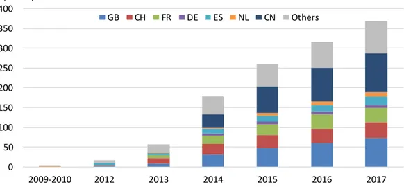
Issuance of CoCo has peaked in 2014 and the cumulative amount of CoCo issuance has reached more than $350 billion as of

2For example, the European Banking Authority provided a term sheet and the Office of the Super- intendent of Financial Institutions Canada published guidelines with respect to the design of CoCos in 2011.

Figure 1.1:

Cumulative Amount of CoCo Issuance

The data show the cumulative amount of issuance of instruments which are labeled as “Contingent Convertible” in Bloomberg. Jurisdictional classification is applied based on the bond domicile (GB:

the United Kingdom except the British Overseas Territories (e.g., Cayman Islands), CH: Switzerland, FR: France, DE: Germany, ES: Spain, NL: the Netherlands, CN: the People’s Republic of China).

Source: Bloomberg.

0 50 100 150 200 250 300 350 400

2009-2010 2012 2013 2014 2015 2016 2017

GB CH FR DE ES NL CN Others (USD bn)

Source: Bloomberg

2017 Q3. Many CoCos have their domiciles in European countries such as the United Kingdom, Switzerland and Germany. CoCo issuance by Chinese banks has also been increasing.

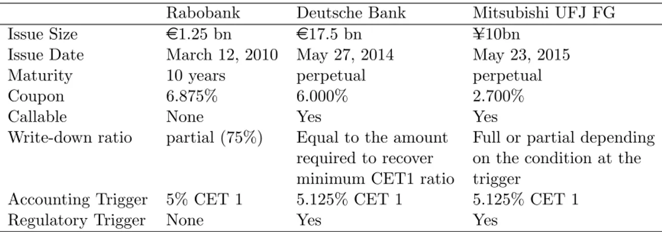
Table 1.1 shows some examples of CoCos in real markets. According to Avdjiev et al. (2017), equity-conversion type CoCos were dominant in early years, but write-down type CoCos have become majority recently.

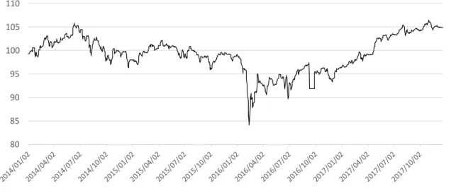
Compared to other major financial instruments, the size of CoCo market is still small. However, the term CoCo was widely noticed in early 2016, when a well-known large banking group in Europe, who had issued CoCos, revealed a huge amount of loss in its statement. As seen in Figure 1.2, the CoCo market experienced a sort of “crush”

at that time. People worried whether the bank had enough strength to afford high-

yield CoCos and questioned whether the risk of CoCos, including ones issued by other

banks, had been evaluated appropriately. Unfortunately, it may be quite challenging

to find a convincing answer to this question since no CoCo has experienced a trigger as

of today. However, recent growth in CoCo markets and the realized crush emphasize

the importance of market participants, as well as regulators, to properly understand

and address risks arising from CoCos.

Table 1.1:

CoCo examples

Equity Conversion

Lloyds Credit Suisse HSBC

Issue Size

$2 bn $2.25 bn

Issue Date December 1, 2009 February 24, 2011 March 24, 2015

Maturity 10-20 years 30 years perpetual

Coupon 6.385-16.125% 7.875% 6.375%

Callable None Yes Yes

Conversion Price fixed floored fixed

Accounting Trigger 5% Core Tier 1 (Basel II) 7% CET 1 7% CET 1

Regulatory Trigger None Yes Yes

(b)

Write-down

Rabobank Deutsche Bank Mitsubishi UFJ FG

Issue Size

1.25 bn

17.5 bn Y =10bn

Issue Date March 12, 2010 May 27, 2014 May 23, 2015

Maturity 10 years perpetual perpetual

Coupon 6.875% 6.000% 2.700%

Callable None Yes Yes

Write-down ratio partial (75%) Equal to the amount Full or partial depending required to recover on the condition at the minimum CET1 ratio trigger

Accounting Trigger 5% CET 1 5.125% CET 1 5.125% CET 1

Regulatory Trigger None Yes Yes

Source:

De Spiegeleer and Schoutens (2012), Prospectus

1.4 CoCos and Regulation

Owing to the loss-absorption mechanism it has, a CoCo is regarded as regulatory capital. Regulatory capital defined in the Basel III framework consists of multiple categories – CET 1, Additional Tier 1, Tier 2 and other buffers. To be brief, Tier 1 and Tier 2 capitals are considered “going-concern” and “gone-concern,” respectively.

In the regulatory context, the term going-concern is often used to emphasize that an instrument is expected to absorb losses in order to continue business operation. On the other hand, there exists a similar but different, so called gone-concern instruments, which are designed to absorb losses upon entry into resolution. This thesis deals with a going-concern type CoCo.

In other words, the trigger level is set equal to or higher

3The Financial Stability Board (2011) requires a regulator to have powers to bail-in an un-triggered CoCo upon entry into resolution. Although we focus on a going-concern feature of a CoCo, in a nutshell, sooner or later, a CoCo is expected to function as a loss-absorbing instrument.

Figure 1.2:

Markit iBoxx USD Contingent Convertible Liquid Developed Markets AT1 In- dex

The index has been calculated daily and rebalanced monthly since December 31, 2013. It is composed of contingent convertibles which are eligible as Additional Tier 1 under the Basel III regulation. As of December 2017, 46 CoCos issued by 21 banking groups are included. Source: Bloomberg, Markit.

80 85 90 95 100 105 110

than the regulatory minimum to ensure business continuity.

Taking into account that a CoCo is a going-concern instrument, it could belong to Tier 1 capital, but it is not always the case. According to the Basel documents, requirements to be counted as Additional Tier 1 include without limitation:

• The issuer has full discretion over payment of a coupon or a dividend.

• The instrument has perpetual maturity and the issuer does not have an incentive to redeem early, including step-up in coupons.

• The instrument could be callable but requires national authority’s approval in advance to exercise the call.

If a CoCo satisfies all the requirements, then it can be classified as Additional Tier 1 capital.

If otherwise, it is labeled as Tier 2 capital.

4Only “pure” capital, which is categorized as “capital” in accounting statements, e.g., common equity and undistributed profits, can be labeled as CET 1 capital. Thus, a CoCo is not a CET 1 instrument.

1.5 Literature

The idea of CoCo was introduced by academic studies such as Flannery (2015), Duffie (2009) and the Squam Lake Working Group

(2009). Regulators such as Bernanke (2009), Dudley (2009) and Haldane (2011) also endorsed to study CoCos by stating that contingent capital would be an option to enhance capital regulation. Since then, there have been many studies on CoCos, especially on valuation using diverse approaches.

Some build their models within the framework of a structural approach, which models bank’s balance-sheet dynamics and is attributed to Merton (1974). Glasserman and Nouri (2012) derive a closed-form solution for CoCos with a capital-ratio trigger by modeling the bank’s asset value process as a geometric Brownian motion. Buergi (2013) proposes a method to price Tier 1 ratio based CoCos by assuming a linear relationship between Tier 1 ratio and disclosed capital ratio. Albul, Jaffee, and Tchistyi (2015) apply Leland (1994) to find an optimal capital structure of a bank issuing CoCo.

De Spiegeleer and Schoutens (2012) propose a credit derivatives approach and an equity derivatives approach to price a CoCo. The former is a straightforward approach that applies a reduced-form model to express the trigger intensity, similarly to the default intensity which is often handled in pricing of credit derivatives. The latter attempts to price a CoCo by using existing barrier-option pricing methods to evaluate cashflow streams that is unique to a CoCo – equity purchase at the trigger and cancel- lation of coupon payments after the trigger. Closed-form solutions are available in both approaches since they consider a stock price, which follows the simple Black-Scholes model, as the trigger indicator.

Chung and Kwok (2015) include a regulatory trigger into their scope. They consider a joint process of stock price and capital ratio, and then apply the structural approach to express an accounting trigger and the reduced-form approach to a regulatory trigger.

Although various models are proposed to evaluate CoCos, there seems to be a mismatch between academic CoCos and actual CoCos from two aspects. First, many studies deal with a single-trigger CoCo, which is often a market trigger or an accounting trigger CoCo, despite the fact that the major trigger mechanism is the combination of an accounting trigger and a regulatory trigger. Some studies include a regulatory trigger into their coverage; however, it may not be sufficient to do an analysis from a regulator’s perspective. Second, continuous-time modeling is often used for the sake of simple calculation although accounting numbers are only available at discrete time (e.g., at the end of each quarter).

5The Squam Lake Group is a group of fifteen academics who offer guidance on the reform of financial regulation.

1.6 Aims of the Study

Aims of the study are to provide a model that can fill in the gap caused by the mis- match and to answer the question that regulators might come up with: “when is the best timing for the regulators to trigger CoCos in practice?” In this thesis, we first model a bank issuing CoCo with an accounting trigger and a regulatory trigger by using a structural-default approach, and then find an optimal capital structure for the bank. We also model a CoCo investor with the structural-default approach and define regulator’s problem. Finally, we look for effective regulatory policy to deal with such CoCos, based on default probabilities of the bank and the investor.

Our contribution can be summarized into three points, all of these issues have not been much addressed in other studies. First, we propose a comprehensive model that includes a CoCo investor and a regulator in addition to a bank. By including an investor into scope, risk contagion, or systemic risks, can also be examined in our model.

Second, we deal with a CoCo that has the trigger mechanism consistent with CoCos in real markets – a combination of an accounting trigger and a regulatory trigger. Finally, we conduct an analysis from regulator’s perspective and suggest effective regulatory policy to handle such CoCo.

This thesis is organized as follows. Chapter 2 is a model description. Numerical

examples using the model are provided in Chapter 3. In Chapter 4, we summarize our

work and derive effective regulatory policy implicated from the numerical examples.

Chapter 2

The Model Setup

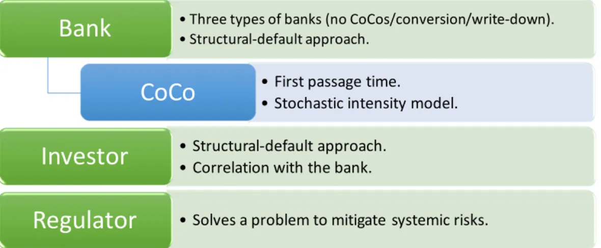
We build a model for each stakeholder – a bank, a CoCo investor and a regulator – respectively. Figure 2.1 provides an overview of our model. A bank model is con- structed within the framework of a structural-default approach, following the idea of studies such as Merton (1974) and Leland (1994). We assume that the CoCo has two types of triggers, i.e., accounting trigger and regulatory trigger. An accounting trigger is expressed in a first-passage-time model, and it happens at periodic disclosure dates.

On the other hand, a regulatory trigger happens upon regulator’s decision, and it is expressed in both first-passage-time and stochastic intensity model. A CoCo investor, which we consider a financial institution, is also modeled by the structural-default ap- proach and has correlation with the bank. In addition, we assume that a regulator solves a problem to mitigate systemic risks, i.e., default probabilities of both bank and investor.

Figure 2.1:

Model Overview

• Three types of banks (no CoCos/conversion/write-down).

• Structural-default approach.

Bank

• First passage time.

• Stochastic intensity model.

CoCo

• Structural-default approach.

• Correlation with the bank.

Investor

• Solves a problem to mitigate systemic risks.

Regulator

2.1 Bank

We consider three types of banks, whose assets are financed by deposits, equity, and a bond or a CoCo:

• Type 0 Bank issues a normal subordinated bond (no trigger mechanism).

• Type 1 Bank issues a CoCo which converts into equity when triggered.

• Type 2 Bank issues a CoCo which suffers a write-down when triggered.

2.1.1 General Framework

First, we illustrate a general framework that can be applied to all three banks, following the idea of Harding et al. (2013) who apply Leland (1994) to obtain firm value of a bank.

We assume that each bank has the same deposit-interest rate d, which is constant and continuously paid to depositors per instantaneous time.

Depositors are protected by the government deposit-insurance scheme and thus the deposits are considered “default- free.” Given a fixed risk-free rate r, value of the deposits D(t) (which must be equal to the face value ¯ D) is given as

D(t) = ¯ D =

∫

0

e

d dt = d

r . (2.1)

Similarly, face value ¯ C of the bond which pays continuous coupon c is equal to C ¯ =

∫

0

e

c dt = c

r . (2.2)

The bank assets V (t) follow geometric Brownian motion under the risk-neutral measure Q , i.e.,

dV (t) = rV (t)dt + σV (t)dz

(t) under Q , (2.3) where V (0) = x. We also consider the process under the physical measure P as reg- ulators are concerned with the “actual” bank-default probabilities. Suppose z

(t) =

−

t + z

(t), it follows that

dV (t) = µV (t)dt + σV (t)dz

(t) under P . (2.4) As banks are subject to the capital regulation and required to maintain minimum capital levels, it is natural to assume that their default conditions are associated with

1Leland (1994) assume that the firm finances the net cost of the debt payment by issuing additional equity. Although this assumption is not practical, we follow Leland (1994) to keep matters analytically tractable.

the capital ratio. Thus, we assume that a bank enters into resolution when its capital ratio falls to a certain fixed level χ

∈ [0, 1). Let Eq(t) be the value of equity disclosed on the balance sheet, then the capital ratio is equivalent to Eq(t)/V (t).

Therefore, the default time τ

can be expressed in a first passage time, i.e.,

τ

= inf {

t ≥ 0; Eq(t) V (t) ≤ χ

}

. (2.5)

We assume that a bank can issue a CoCo which has an accounting trigger and a regulatory trigger. An accounting-trigger condition can be defined similarly to the default condition by using the capital ratio Eq(t)/V (t). If we assume a continuous-time accounting trigger, i.e., a trigger may happen at any instantaneous time, the trigger time denoted as τ

can be expressed as

τ

= inf {

t ≥ 0; Eq(t) V (t) ≤ χ

}

, (2.6)

where χ

∈ (χ

, 1) is the trigger level. The condition χ

> χ

must be satisfied to ensure going-concern loss absorption. Otherwise, the bank enters into resolution before the trigger event to take place.

In practice, however, accounting numbers are only disclosed periodically, for in- stance, quarterly or annually. Thus, we need to think of a discrete-time account- ing trigger, i.e., triggers can only happen at periodic disclosure dates.

Assume that T

, n ∈ N is a calculation date of the capital ratio, the trigger time τ

is defined as

τ

= inf {

T

; n ∈ N , Eq(T

) V (T

) ≤ χ

}

. (2.7)

Next, we define a model for a regulatory trigger. The regulatory trigger happens depending on the regulator’s discretion, but of course it does not come haphazardly; a regulator would exercise the right to trigger the CoCo when some sort of “insolvency sign” is found. Thus, we need to think of a model that is associated with some signs in order to express the regulatory trigger. The sign could be induced by either (1) factors

2To be precise,V(t) is the “market” asset value and it should not be equal to the “book-value” of the assets. However, according to Buergi (2013), the book-value of assets can be approximated by its market value when the financial condition is severe, as accounting standards support “the conservatism principle.” Under the principle, the lower of cost or market rule is applied, thus market value is more likely to be disclosed during the stress period.

3Banks may calculate the amount of regulatory capital more often when its financial condition become severe, but it may still take certain time to obtain confirmed numbers at the group consolidated level when we consider a SIFI, who is operating globally. Thus, it is more realistic to assume the discrete-time accounting trigger rather than the continuous one.

other than the asset value (e.g., liquidity of assets)

or (2) the asset value itself.

The first one can be modeled by applying a stochastic intensity model, following the idea of Chung and Kwok (2015);

τ

= inf {

t ≥ 0;

∫

h(V (u))du ≥ X }

, (2.8)

where h is a trigger-intensity function and X is an exponentially distributed random variable independent of the Brownian motion z

(t). Given an appropriate function h, the above formula makes τ

to follow a Cox process. Hereinafter, the expectation at time t conditional on V (0) = x under the measure Q is denoted as E

[ · ] for brevity (t could be omitted when t = 0). Under the Cox process, the probability of the trigger to take place within some risk horizon t is given by

Q{ τ

< t } = Q {∫

0

h(V (s))ds ≥ X }

= 1 − E

[

e

]

. (2.9)

Although any function that satisfies h(t) ≥ 0 and ∫

0

h(t)dt = ∞ works as an intensity function, here we suppose that h is a non-increasing function with regard to the asset value V (t). The rationale behind this is that the factor generating the insolvency sign should have negative correlation with the asset value. To be more specific, when the market condition become severe, market liquidity decreases and pushes up the trigger- intensity; at that time, the asset value V (t) is also in the decreasing phase. Thus, if we look at the relationship between h and V (t), we can say that they should have negative correlation.

The second regulatory trigger is modeled by the first passage time, i.e., τ

= inf

{

t ≥ 0; V (t) + ϵ ≤ V

}

, (2.10)

where ϵ is a Gaussian noise with 0 mean and the standard deviation being given by σ

. The noise indicates that regulators are monitoring the approximate asset value as the exact amount of V (t) cannot be obtained at time t.

4OSFI (2011) announces the criteria that the OSFI (the Superintendent) may consider when they trigger a CoCo issued by a deposit-taking institution (DTI) under its supervision. The criteria include but not limited to:

• “Whether the assets of the DTI are, in the opinion of the Superintendent, sufficient to provide adequate protection to the DTI’s depositors and creditors.”

• “Whether the DTI has lost the confidence of depositors or other creditors and the public. This may be characterized by ongoing increased difficulty in obtaining or rolling over short-term funding.”

• “Whether the DTI’s regulatory capital has, in the opinion of the Superintendent, reached a level, or is eroding in a manner, that may detrimentally affect its depositors and creditors.”

The second trigger defined in (2.10) is a key element in our model, because it enables an analysis from the regulator’s perspective. Although (2.8) is one reasonable way to express a regulatory trigger, it is totally “stochastic” because X is a random variable.

On the other hand, (2.10) is considered a “controllable” trigger as it is possible to set the level of V

in alignment with the regulator’s strategies. For example, if we suppose a relatively low V

, it indicates that the regulator is not willing to trigger the CoCo unless the bank faces undoubtedly severe financial condition.

Having set all the necessary triggers, the trigger time τ

can be obtained by τ

= min { τ

, τ

, τ

} . (2.11) Given the fact that even “a possibility of a trigger” had a considerable impact on market volatilities in early 2016, we should make a presumption that “an actual trigger” may have even larger impact. To express this, we assume that the trigger event changes the volatility of the bank asset-value process, i.e.,

dV (t) = rV (t)dt + σV (t)dz

(t), t ∈ [0, τ

), (2.12) dV (t) = rV (t)dt + σ

V (t)dz

(t), t ∈ [τ

, ∞ ). (2.13) It is reasonable to assume that the trigger makes the asset process more volatile, i.e., σ < σ

. The reason behind this assumption is as follows; as the fact, a trigger of CoCo delivers the information that the bank has been facing a financial difficulty. Although its capital ratio recovers by the trigger, taking into account that less historical evidence is available to be convinced that the bank can fully turn around, it is more likely that the trigger of CoCo weakens the bank’s credibility among market participants. The bank may suffer a higher funding costs due to less credibility, and forced to do some riskier investments to attain higher expected returns to meet the costs, which results in larger asset volatility.

Having provided all the necessary conditions, finally we define the total value of the bank, denoted as v (x),

v(x) = x − B(x) + F (x) + I (x), (2.14) where B , F and I stand for bankruptcy costs, franchise value and insurance benefits, respectively. Specific expressions for each term are provided in the following subsec- tions, as they differ according to the type of the bond issued.

2.1.2 Type 0 Bank (Subordinated Bond)

Type 0 Bank issues a normal subordinated bond, not a CoCo (thus, for the time being,

the above trigger mechanism can be ignored). Its capital structure (i.e., deposits,

the bond and equity on the credit side) does not change throughout its life. Hence,

V (t) = ¯ D + ¯ C + Eq(t) must be satisfied for ∀ t ≤ τ

.

Hence, Equation (2.5) can be rewritten as

τ

= inf { t ≥ 0; V (t) ≤ V

} , where V

=

D ¯ + ¯ C

1 − χ

. (2.15) When a bankruptcy occurs, the bank enters a liquidation process which obliges the bank to pay bankruptcy costs (e.g., judicial costs). Here we assume that the bankruptcy costs are proportionate α ∈ (0, 1) of the asset value at time τ

, thus equal to αV

. Hence, B (x) is expressed as

B(x) = αV

E

[ e

]

. (2.16)

As long as the bank is solvent, the bank benefits from the debt financing (e.g., tax benefit) and we call this the franchise value. We assume that the benefit is proportional to the payment generated from the debt financing, which is equal to d + c. Given the proportional factor δ ∈ (0, 1), the franchise value F (x) become

F (x) = E

[∫

0

e

δ(d + c)dt ]

= δ( ¯ D + ¯ C) (

1 − E

[ e

])

. (2.17)

The residual assets after the bankruptcy, (1 − α)V

, is allocated to the depositors. If not sufficient to compensate all the deposits ¯ D, the gap is refunded from the deposit- insurance fund. Hence, the value protected by the deposit-insurance scheme equals to

max { D ¯ − (1 − α)V

, 0 }

. (2.18)

In practice, it is reasonable to assume max { D ¯ − (1 − α)V

, 0 }

̸

= 0, otherwise it is meaningless to think of a deposit-insurance scheme. Thus, under the assumption that the value of the protection is not zero, the insurance benefits I(x) become

I(x) = ( ¯ D − (1 − α)V

) E

[ e

]

. (2.19)

Given τ

defined in Equation (2.5), we can prove that E

[

e

]

= ( x

V

)

(2.20) where γ = 2r/σ

. The proof is provided in Appendix A. Hence, by collecting above, the firm value of Type 0 Bank at t = 0 can be expressed analytically as

v (x) = x + δ( ¯ D + ¯ C) (

1 − ( x

V

)

)

+ ( ¯ D − V

) ( x

V

)

. (2.21)

Next, we evaluate the market value of the bond. Recall that we are considering a subordinated bond, the residual assets after the bankruptcy are reimbursed to de- positors first and then to the bond holders, if any. Thus, the value of recovery equals to

min { C, ¯ max { (1 − α)V

− D, ¯ 0 }} . (2.22) In practice, though, it is realistic to suppose that the value of recovery is usually 0. If otherwise, it implies that there exists plenty amount of assets left at the time of default, thus no need to put deposit-insurance scheme to practical use. With no recovery, the value of the bond C(V (t)) is expressed as

C(V (t)) = E

[∫

t

e

c ds ]

= ¯ C (

1 − E

[ e

])

, (2.23)

which indicates from Equation (2.20) that C(V (t)) also has an analytic expression.

2.1.3 Type 1 Bank (Equity-Conversion CoCo)

We now consider Type 1 Bank, who issues an equity-conversion type CoCo. We assume that the full amount of the CoCo converts into equity, the value of which is equal to λ C, ¯ λ ∈ R +. Thus, λ can be interpreted as a conversion ratio. For example, in the case of λ = 0.5, it indicates that the CoCo investor receives some stocks at the trigger moment, but value of which only equals to the half of the face value of the original CoCo.

Hence, the market value of the CoCo is given by C(V (t)) = E

[∫

t

e

c ds + e

λ C ¯ ]

= ¯ C(1 − E

[ e

]

) + λ C ¯ · E

[ e

]

. (2.24)

As shown in Figure 2.2, the capital structure of the bank changes as a result of the trigger. Consequently, the balance sheet condition for Type 1 Bank is V (t) = D ¯ + ¯ C + Eq(t) if t ≤ τ

, and V (t) = ¯ D + Eq(t) otherwise. From (2.5) and (2.7), we obtain

τ

= inf { t ≥ 0; V (t) ≤ V

} , where V

= D ¯ 1 − χ

, (2.25)

τ

= inf { T

; n ∈ N , V (T

) ≤ V

} , where V

=

D ¯ + ¯ C

1 − χ

. (2.26)

The bankruptcy costs and the insurance benefits are the same as those of Type 0 Bank,

defined as (2.16) and (2.19), respectively. On the other hand, the amount of payment

Figure 2.2:

Capital Structure of Type 1 Bank

Asset

%(')

Deposit -.

CoCo (Conversion) 3. Equity

89(')

Asset

%(')

Deposit -.

Equity 89(')

Trigger

generated from the debt financing is reduced from d + c to d after the conversion; thus the expression for F (x) differs, i.e.,

F (x) = E

[∫

0

e

δd ds +

∫

0

e

δc ds ]

= δ D ¯ (

1 − E

[ e

])

+ δ C ¯ (

1 − E

[ e

])

. (2.27)

Now let’s consider how we can calculate the firm value v (x) in the case of Type 1 Bank. If we assume that the CoCo only has the continuous-time accounting trigger, a closed-form solution is available, provided that

E

[ e

]

= E

[ e

]

= ( x

V

)

, t ≤ τ

, (2.28) and

E

[ e

]

= E

[ e

]

· E

[ e

]

= ( x

V

)

(

V

V

)

, t ≤ τ

(2.29)

where γ

= 2r/(σ

)

. The proof is provided in Appendix A. The second equation in (2.29) follows from the strong Markov property of the Brownian motion.

Unfortunately, if we consider the case of the trigger defined in (2.11), which we aim to discuss in this thesis, the story is not as simple as above – an analytic solution is not available. Instead, we can formulate an integral equation with regard to v(x), which is

v(x) = E

[

e

v(V (T ))1

] + E

[

e

v

(V (T ))1

] + E

[

e

v

(V (τ

))1

]

, (2.30)

where τ

= min { τ

, τ

} and v

(V (t)) is the firm value calculated under the asset- value process after the trigger as defined in Equation (2.13).

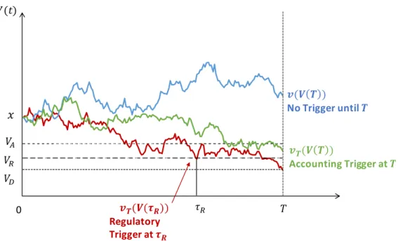
Here we provide a narrative description on how this equation can be constructed. If we consider only one period of time until the next capital-ratio evaluation date denoted as T , one of the following three cases would happen:

1. The bank experiences no trigger until T , thus the bank structure is unchanged and the firm value at T equals to v(V (T )).

2. An accounting trigger takes place at T , while regulatory triggers have not emerged.

In this case, the firm value at T is expressed as v

(V (T )) because the asset-value process changes to (2.13).

3. A regulatory trigger happens somewhere in [0, T ), resulting in the firm-value function to change from v to v

starting at τ

.

Figure 2.3 shows an image of the above description. By taking expectation and dis- counting each of the three terms, we obtain the current firm value v (x).

The function v

(V (t)) can be obtained explicitly. Suppose that V (t) = y. It follows that

v

(y) = y + δ D ¯ (

1 − ( y

V

)

)

+ ( ¯ D − V

) ( y

V

)

. (2.31)

It appears that the above equation is quite similar to (2.21), the firm value of Type 0 Bank. It is not surprising because Type 1 Bank after conversion and Type 0 Bank share the same features – the asset-value process following geometric Brownian motion (no volatility change expected in the future) and the default condition expressed in the first passage time (expressions of V

are different, though).

To solve (2.30), numerical calculation is available for some parts, yet not fully applicable. We can use Monte-Carlo simulation to make up for the residual calculation;

however, it is not straightforward as it involves rare-event simulation. More details are provided in Appendix B.

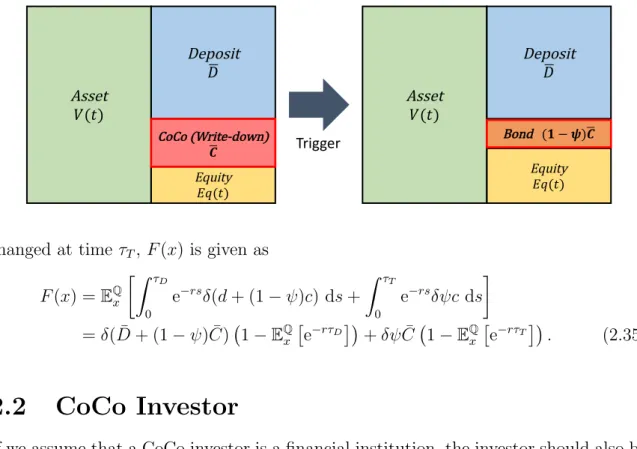
2.1.4 Type 2 Bank (Write-down CoCo)

Type 2 Bank issues a write-down type CoCo. At the trigger event, a fraction ψ ∈ [0, 1]

of the CoCo suffers a write-down as shown in Figure 2.4. We assume that a part of the CoCo that has not been written-down stays in its balance sheet as a normal subordinated bond.

Accordingly, the balance-sheet condition for Type 2 Bank is

5In practice, the issuer may redeem the part of CoCo that has not suffered a write-down rather than keeping them on its balance sheet as a normal bond. However, early redemption has the same impact as the equity conversion in the sense that they both provide a certain fixed value to the investor at the trigger. Thus, no redemption is assumed in our model.

Figure 2.3:

Firm-Value Calculation

𝑥

𝑉_$ 0 𝑉(𝑡)

𝒗_𝑻(𝑽(𝝉_𝑹)) Regulatory Trigger at 𝝉_𝑹 𝑉_-

𝒗(𝑽 𝑻 )

No Trigger until 𝑻

𝒗_𝑻(𝑽 𝑻 )

Accounting Trigger at 𝑻

𝜏_- 𝑇

V (t) = ¯ D + ¯ C + Eq(t) if t ≤ τ

, and V (t) = ¯ D + (1 − ψ) ¯ C + Eq(t) otherwise, which derives

τ

= inf { t ≥ 0; V (t) ≤ V

} , where V

=

D ¯ + (1 − ψ) ¯ C

1 − χ

, (2.32) τ

= inf { T

; n ∈ N , V (T

) ≤ V

} , where V

=

D ¯ + ¯ C

1 − χ

. (2.33) The market value of the write-down type CoCo is given by

C(V (t)) = E

[∫

t

e

(1 − ψ)c ds +

∫

t

e

ψc ds ]

= (1 − ψ) ¯ C(1 − E

[ e

]

) + ψ C ¯ (

1 − E

[ e

])

. (2.34) If we consider the case of ψ = 0, we see that (2.34) becomes (2.23), which is not surprising as ψ = 0 indicates no write-down at the trigger event thus the bond can be considered a normal subordinated bond. On the other hand, ψ = 1 makes (2.34) to be the same as (2.24) given λ = 0. It implies that the write-down type CoCo takes a middle position between the subordinated bond and the equity-conversion type CoCo.

The bankruptcy costs and the insurance benefits are the same as those of the other

banks. As for the franchise value, bear in mind that the amount of debt payment has

Figure 2.4:

Capital Structure of Type 2 Bank

Asset

%(')

Deposit -.

CoCo (Write-down) 6.

Equity

;<(')

Asset

%(')

Deposit -.

Equity

;<(')

Trigger Bond (? − A)6.

changed at time τ

, F (x) is given as F (x) = E

[∫

0

e

δ(d + (1 − ψ)c) ds +

∫

0

e

δψc ds ]

= δ( ¯ D + (1 − ψ) ¯ C) (

1 − E

[ e

])

+ δψ C ¯ (

1 − E

[ e

])

. (2.35)

2.2 CoCo Investor

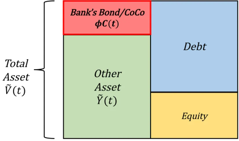
If we assume that a CoCo investor is a financial institution, the investor should also be included in the analysis scope as regulators are concerned with its behavior to prevent systemic risks. In the same way as banks, we apply the structural-default approach to model a CoCo investor who possesses a certain fraction ϕ ∈ [0, 1] of a bond/CoCo issued by the bank.

Figure 2.5 shows the capital structure of the investor. As indicated, the investor has the certain amount of the bond or CoCo issued by the bank, ϕC(t), and the other assets denoted as Y e (t). In the case of an investor who buys the bond issued by Type 0 Bank, Y e (t) follows

d Y e (t) = ϕc1

dt + µ e Y e (t)dt + σ e Y e (t)d e z

(t). (2.36) where 1

is an indicator function (equals to 1 if A is true and 0 otherwise) and z e

(t) is a Brownian motion under the measure P , which has correlation ρ with z(t); thus

dz

(t)d e z

(t) = ρ dt. (2.37) For an investor who buys a CoCo issued by Type 1 Bank, Y e (t) follows

d Y e (t) = ϕc1

dt + ϕλ C1 ¯

+ µ e Y e (t)dt + e σ Y e (t)d e z

(t). (2.38)

Figure 2.5:

Capital Structure of Investor

Other Asset

)*(,)

Debt

Bank’s Bond/CoCo 9:(;)

Equity

Total Asset

C*(,)

Finally, the process of Y e (t) for an investor having Type 2 Bank CoCo is

d Y e (t) = ϕc1

dt + ϕ(1 − ψ)c1

dt + µ e Y e (t)dt + e σ Y e (t)d z e

(t). (2.39) The idea here is that Y e (t) basically follows a geometric Brownian motion – the last two terms on the RHS of (2.36), (2.38) and (2.39), – and relevant income generated from the bond or the CoCo (e.g., coupon, amount of stocks received at the conversion) is added to the process. For example, in the case of Type 1 Bank, the first and the second terms on the RHS of (2.38) indicate that the investor earns coupon ϕc until the trigger moment and receives shares which have the value equals to ϕλ C ¯ at the trigger moment.

Let us denote the investor’s total assets by V e (t). Taking into account that the asset side of the investor changes at the event of trigger or default of the bank, V e (t) is equivalent to

Type 0 Bank investor: V e (t) =

{ Y e (t) + ϕC(V (t)), 0 ≤ t < τ

,

Y e (t), τ

≤ t, (2.40)

Type 1 Bank investor: V e (t) =

{ Y e (t) + ϕC(V (t)), 0 ≤ t < τ

,

Y e (t), τ

≤ t, (2.41)

Type 2 Bank investor: V e (t) =

 



 

Y e (t) + ϕC(V (t)), 0 ≤ t < τ

, Y e (t) + ϕ(1 − ψ)C(V (t)), τ

≤ t < τ

,

Y e (t), τ

≤ t.

(2.42)

Provided that the investor is also a financial institution, it is reasonable to assume that

its default condition is also fixed by some kind of regulation; we define the investor’s

default time τ e

as

e

τ

= inf { t ≥ 0; V e (t) ≤ χ e

} (2.43) where χ e

is an exogenous constant indicating a default barrier.

2.3 Regulator

A regulator has the right to trigger a CoCo issued by the bank under its supervision.

Specific criteria on when and how the regulator determines the trigger is not made public. However, we can define some reasonable “mechanism” to determine the regu- latory strategy, by paying attention to the fact that regulators act to prevent systemic risks.

It may be possible to express the systemic risks in several ways, e.g., joint default- probabilities of the bank and the investor. In this study, however, we put more focus on the bank’s default probability compared to the investor’s. Namely, we define the regulator’s problem as

min

P{ τ

< T } (2.44)

subject to P{e τ

< T | τ

< e τ

, τ

< T } < p, ¯ (2.45) where T is a risk horizon set by the regulator. Explanations for ¯ c and ¯ p are provided later in this chapter.

(2.45) is the investor-default probability conditional on a trigger event to happen before default of the investor. This implies that the regulator would not allow investor- default probability to become higher than a certain level, denoted as ¯ p. Hence, ¯ p can be interpreted as a “breaking point” of a stable financial system, i.e., the financial system is no longer resilient if the investor-default probability becomes higher than the threshold ¯ p.

The problem indicates that regulator’s main objective is to mitigate bank-default risks, but investor’s default risk is also taken into account as a constraint. To begin with, a CoCo is invented to enhance the resilience of the bank; thus it is reasonable to assume that the regulator triggers the CoCo if necessary to recover the bank capital.

However, we should not consider bank default risks “only” because an eventual goal that regulators bear in mind is the resilient financial system as a whole, which should include CoCo investors. Thus, the regulator is also responsible for preventing investors from suffering an unendurable loss due to the CoCo.

We assume that the regulator can control the level of V

defined in (2.10). In

addition, we add another controllable parameter, which is an issuance limit ¯ c. The

issuance limit is a regulation imposed to banks; under the limit, banks are not allowed to issue a CoCo if its coupon c does not fall within the range of c ∈ [0, ¯ c].

6In practice, it may be difficult for regulators to directly restrict the level of coupons. However, there exist some regulations that indirectly limits the amount of CoCo issuance. For example, a minimum requirement for CET 1 ratio works as a restriction against CoCo issuance because CoCos are not included in the CET 1 capital.