Point-condensation phenomena and saturation eﬀect for the Gierer-Meinhardt system ギーラー・マインハルト系における

(1)

Point-condensation phenomena and saturation eﬀect for the Gierer-Meinhardt system ギーラー・マインハルト系における

点凝集現象と飽和効果 ( 英文 )

Kotaro Morimoto

森本光太郎

(2)

Background and main results

In this thesis, we will study some systems of nonlinear partial diﬀerential equations arising as models of a biological pattern formation or a chemical reaction.

We are mainly concerned with the Gierer-Meinhardt system which is a model of an activator and an inhibitor in the ﬁeld of biological pattern formation.

The most fundamental problem in morphogenesis is how an inhomogeneous pattern is constructed. A. Gierer and H. Meinhardt (1972) explained the phenomenon by using two biochemical substances an activator and an inhibitor, and they proposed a model equation of the activator and the inhibitor in the form of a reaction-diffusion system. Today, the model equation is called the Gierer-Meinhardt system. In this thesis, we will mainly study the steady-state problem of the Gierer-Meinhardt system. The analytical methods which will be used to construct solutions to the Gierer-Meinhardt system also work for other models so-called the Schnakenberg model and the chemotaxis model. We will investigate the “point-condensation phenomena” and the “saturation effect” for each model. Let us state the background of our study and main results of this thesis (Theorems A-G). We first introduce a reaction-diffusion system.

1.1 Reaction-diﬀusion system

In general, the n-component reaction-diﬀusion system is described as follows:

 

 

 

 



∂u1

∂t

= d

1

∆u

1

+ f

1

(u

1

, · · · , u

n

) in Ω, t > 0,

∂u₂

∂t

= d

₂

∆u

₂

+ f

₂

(u

₁

, · · · , u

_n

) in Ω, t > 0, .. .

∂un

∂t

= d

n

∆u

n

+ f

n

(u

1

, · · · , u

n

) in Ω, t > 0,

(1.1)

(5)

where Ω is a bounded domain in R

^N

with smooth boundary ∂Ω. ∆ is the Laplace operator in R

^N

, namely,

∆ =

∑

N j=1

∂

²

∂x

²_j

.

Each u

_i

(x, t), i = 1, · · · , n, denotes the concentration or density of a single species in isotropic diﬀusitive medium at time t and position x. d

i

> 0, i = 1, · · · , n, denotes the diﬀusion constant of u

i

. The boundary and initial conditions are

∂u

i

∂ν = 0 on ∂Ω, (1.2)

u

i

(x, 0) = a

i

(x) in Ω, (1.3) for i = 1, · · · , n, where ν is the outer normal vector on the boundary. The condition (1.3) is called a homogeneous Neumann boundary condition or zero ﬂux boundary condition. The each term f

i

(u) is called a reaction term of u

i

. In the ﬁelds of chemistry, ecology and biology, a lot of models described in the form (1.1) have been proposed.

1.1.1 Scalar reaction-diﬀusion equation

When n = 1 for (1.1), it is particularly called a scalar reaction-diﬀusion equation:

∂u

∂t = d∆u + f (u) in Ω, t > 0, (1.4)

∂u

∂ν = 0 on ∂Ω, u(x, 0) = a(x) in Ω.

(1.5) Formally, the equation (1.4) consists of the following well-known equations:

∂u

∂t = d∆u, (1.6)

∂u

∂t = f (u). (1.7)

(1.6) is a simple diffusion equation (or heat equation). The diffusion equation (1.6) describe the diffusion-phenomena of diffusitive substances. If we consider the problem (1.6) under the conditions (1.5), then it is known that

t

lim

→∞

u(x, t) = 1

| Ω |

∫

Ω

a(x)dx. (1.8)

That is, by the eﬀect of diﬀusion, u(x, t) tends to the average of its initial data

(see e.g. [99]). The fact is very natural. On the other hand, if we consider u to

(6)

be independent of x, namely, u(x, t) = u(t), then the reaction of u is described by the kinetic equation (1.7). We note that, if the algebraic equation

f (u) = 0, u ∈ R ,

has a solution u

c

∈ R , then it is also a constant solution of (1.4). By the analogy from the heat equation, we can similarly expect that any solution of (1.4) tends to a uniform state, namely, some constant solution u

c

. This expectation is true when d is large enough (see [12]). Moreover, the following facts are known for (1.4)-(1.5):

(i) The ω-limit set consists of equilibrium solutions only [32].

(ii) If the domain Ω is convex, any nonconstant solutions are unstable, even if they exist [10, 58].

(iii) There are suitable nonconvex domain Ω and f (u) such that there exists stable nonconstant equilibrium solutions [58].

Here, an equilibrium solution (or a stationary solution, a steady-state solution) is a solution which is independent of time t, that is, u(x, t) = u(x), and it satisﬁes

0 = d∆u + f (u) in Ω, ∂u

∂ν = 0 on ∂Ω. (1.9)

The results (i)-(iii) indicate that any bounded solution generically approaches one of the stable constant solutions provided the domain Ω is convex. This result is also natural because the diﬀusion enhances spatial homogeneity. Therefore, it was long believed that a phenomenon which is described by reaction-diﬀusion systems were not interesting from pattern formation viewpoints. However, the situation turned by Turing’s suggestion.

1.1.2 Diﬀusion-induced instability

In 1952, A. Turing [102] insisted that diﬀusion enhances spatial inhomogeneities.

His insistence was surprising then because many mathematicians believed that diffusion enhances spatial homogeneities. The key of his insistence is that, for two diffusivity substances, let their diffusion-rate be different widely, then the homogeneous steady-state may become unstable. He indeed demonstrated it by using some linear model. Today, it is called diffusion-induced instability or Turing instability. Although his model is linear, his idea is naturally extended to the nonlinear model as two-component reaction-diffusion systems:

{

∂u₁

∂t

= d

₁

∆u

₁

+ f

₁

(u

₁

, u

₂

) in Ω, t > 0,

∂u₂

∂t

= d

2

∆u

1

+ f

2

(u

1

, u

2

) in Ω, t > 0, (1.10)

with zero ﬂux boundary condition. By many mathematicians, for suitable re-

action terms f

1

and f

2

, the diﬀusion-induced instability was substantiated in

mathematical and numerical way. One of the popular model which realizes the

diﬀusion-induced instability is the Gierer-Meinhardt system.

(7)

1.2 Gierer-Meinhardt system

One of the models which realize the Turing instability is the activator-inhibitor model which was proposed by A. Gierer and H. Meinhardt [22]. An activator and an inhibitor are biochemical substances and are supposed to be satisﬁed the following conditions:

(i) Activator grows in an autocatalytic way.

(ii) Activator produces also inhibitor.

(iii) Inhibitor inhibits activator’s growth.

Under these conditions, Gierer and Meinhardt proposed the following reaction- diﬀusion system which is called the Gierer-Meinhardt system:

 

 



 

 

∂A

∂t

= ε

²

∆A − A +

_H_q_(1+κA^A^p _p₎

+ σ

₀

, A > 0 in Ω × (0, ∞ ), τ

^∂H_∂t

= D∆H − H +

_H^A^rs

, H > 0 in Ω × (0, ∞ ),

∂A

∂ν

=

^∂H_∂ν

= 0 on ∂Ω × (0, ∞ ),

A(x, 0) = A

0

(x), H(x, 0) = H

0

(x) in Ω,

(1.11)

where ε > 0, τ > 0, κ ≥ 0. Ω is a bounded domain in R

^N

(N ≥ 1) with smooth boundary ∂Ω. A = A(x, t) and H = H (x, t) represent the concentrations of the activator and the inhibitor at x ∈ Ω and t ∈ (0, ∞ ), respectively. A

₀

and H

₀

are their initial data. ε and D stand for the diﬀusion constants of the activator and the inhibitor, respectively. The constant κ stands for the degree of saturation eﬀect. The term σ

₀

= σ

₀

(x) is a source term which means a source rate of the activator. The exponents are assumed to be satisﬁed p > 1, q, r > 0, s ≥ 0, and 0 < (p − 1)/q < r/(s + 1). This assumption ensures the existence of a (unique) constant solution to (1.11). For this system, it is known that the constant solution becomes unstable when ε

²

<< D (diﬀusion-induced instability) even if it is stable when ε

²

and D are not so diﬀerent.

We will see that the Gierer-Meinhardt system has various kinds of stationary solutions and that the stability depends on the parameters. In this thesis, we will address the saturation eﬀect, namely, the parameter κ. We ﬁrst introduce some interesting investigations for the Gierer-Meinhardt system of no saturation case κ = 0.

1.2.1 Shadow system of the Gierer-Meinhardt system without saturation

We ﬁrst introduce a limit system of the Gierer-Meinhardt system which was

proposed by Nishiura [80]. By taking the limit D → ∞ formally after dividing

the second equation of (1.11) by D, we have ∆H = 0 and

^∂H_∂ν

= 0 on ∂Ω. Then

we notice that H(x, t) is spatial homogeneous, namely, H (x, t) = ξ(t), and we

(8)

obtain a system for A(x, t) and ξ(t) which is called the shadow system of the Gierer-Meinhardt system:

 



 

∂A

∂t

= ε

²

∆A − A +

_ξ_q_(1+κA^A^p _p₎

+ σ

₀

, A > 0 in Ω, t > 0, τ

^∂ξ_∂t

= − ξ +

_|_Ω¹_|_ξ_s

∫

Ω

A

^r

dx, ξ > 0, t > 0,

∂A

∂ν

= 0 on ∂Ω, t > 0.

(1.12)

Let κ = 0 and σ

0

= 0. Let us consider stationary solutions of (1.12). If we put A(x) = ξ

^q/(p⁻¹⁾

u(x), (1.13) and substitute this into the steady-state shadow system of (1.12), then we have the following equations for (u, ξ):

{

ε

²

∆u − u + u

^p

= 0 in Ω,

∂u

∂ν

= 0 on ∂Ω, (1.14)

ξ

^γ

= ∫ | Ω |

Ω

u

^r

(x)dx , (1.15)

where γ := qr/(p − 1) − (s + 1) > 0. Therefore, we notice that, if we get a solution to (1.14), then deﬁning ξ by (1.15) we obtain a stationary solution to the shadow system (1.12) in the case κ = 0 and σ

0

= 0.

Let us consider the scalar reaction-diﬀusion equation corresponding to (1.14):

 



 

∂u

∂t

= ε

²

∆u − u + u

^p

in Ω, t > 0,

∂u

∂ν

= 0 on ∂Ω, t > 0, u(x, 0) = u

0

(x) in Ω.

(1.16)

If we consider the diﬀusionless equation of (1.16), the ordinary diﬀerential equation is given by {

_du(t)

dt

= − u(t) + u

^p

(t), t > 0,

u(0) = u

0

. (1.17)

Note that this ODE has two equilibrium solutions u = 0, 1, and u = 0 is stable, while u = 1 is unstable. When the domain Ω is convex, one easily knows that a stable stationary solution to (1.16) is u = 0 only. Moreover, it is known that (1.16) loses all its stationary solutions except the trivial ones u = 0, 1 when ε is large (see [53]).

Let us consider the case where ε is small. In the case N = 1, a lot of works have been done by I. Takagi [101]. In the case N ≥ 2, the situation becomes more interesting. By W.-M. Ni et al. [53, 75, 76], a nonconstant stationary solution to (1.14) was constructed for suﬃciently small ε by the variational approach due to the Mountain Pass Theorem, namely, so-called a least-energy solution to (1.14), under the restriction:

1 < p < ∞ if N = 1, 2, 1 < p < N + 2

− if N ≥ 3. (1.18)

(9)

Moreover, they showed that the least-energy solution is concentrated at only one point on the boundary. More precisely, for ε suﬃciently small, the least- energy solution attains its maximum only on one point P

ε

∈ ∂Ω. Moreover, H(P

ε

) → max

P∈∂Ω

H(P ) as ε → 0 holds, where H (P) is a mean curvature function with respect to the inner normal of the boundary ∂Ω. If Ω is convex, then H (P ) ≥ 0. By using the least-energy solution to (1.14), we obtain a stationary solution, so-called a least-energy pattern, to the shadow system (1.12) in the case κ = 0, σ

₀

= 0. It is known that, for suﬃciently small τ, the least- energy pattern is weakly stable if r = p+1 holds, and it is stable if the domain Ω is an annulus (see [78]). Such a spiky-shaped solution is called a peak solution or a spike-layer solution. Although the least-energy solution to (1.16) was a single peak solution, after their work, multi-peak solutions were constructed by many authors. For boundary peaks see [29, 107, 17, 26, 50, 110], for interior peaks see [27, 108, 41], for mixed boundary and interior peaks see [28], and the references therein. By their works, multi-peak solutions to the shadow system (1.12) in the case κ = 0 and σ

0

= 0 were established. However, it seems that multi-peak solutions to the shadow system are unstable. Indeed, Y.

Nishiura [81] and W.-M. Ni, P. Pol´ aˇ cik and E. Yanagida [73] proved that, for the one-dimensional shadow systems with Ω = (0, 1), only monotone stationary solutions could be stable. In the case N = 2, Y. Miyamoto [63] showed that, for two-dimensional shadow system, if Ω is a disc in R

²

, then a stationary solution (A, ξ ) which has more than two peaks at the boundary is unstable. Moreover, it was proven by F. Li, K. Nakashima and W.-M. Ni [52] that, if Ω is a convex domain in R

^N

with smooth boundary, then a non-constant stationary solution (A, ξ ) is unstable for all large τ. In addition, they showed that, if N ≥ 2 and Ω is a ball or an annulus, then a non-constant radially symmetric stationary solution (A, ξ) is unstable. Recently, K. Ikeda, S. Ei and E. Yanagida proved that multi-peak solutions to the shadow system are always unstable for general domains. Namely, stationary peak solutions which has k-peaks (k ≥ 2) on Ω are always unstable. In W.-M. Ni’s survey paper [71], one can ﬁnd some results on the qualitative properties for some elliptic problems such as (1.16).

1.2.2 Main result: instability result for the shadow system

One of main results in this thesis is on the instability for some solutions to the shadow system (1.12) on cylindric domains. Let Ω be a cylindric domain in R

^N

such that Ω = G × ( − T, T ) where G is a smooth bounded domain in R

^N⁻¹

and T ∈ (0, ∞ ). Then we have the following result:

Theorem A. Suppose that p = r − 1 and κ = σ

0

= 0 in (1.12). Let (A(x), ξ) be a stationary solution to (1.12). If A(x) is symmetric with respect to the x

N

-direction, i.e., A(x

⁰

, x

N

) = A(x

⁰

, − x

N

) for (x

⁰

, x

N

) ∈ Ω, and

_∂x^∂A

N

6≡ 0, then (A(x), ξ) is unstable for all τ > 0.

Actually, we can show the result above for more general shadow system. For

more precise statement, see Chapter 9.

(10)

1.2.3 Solutions of the full system without saturation

As we observed, a lot of stationary solutions to the shadow system have been constructed. However, to construct stationary solutions to the full system (1.11) is more diﬃcult than the shadow system. We mention in the case κ = 0.

(Solutions near the shadow system with κ = 0) In some cases, solutions to the full system can be constructed near the one to the shadow system for sufficiently small ε and sufficiently large D. In the case N = 1, I. Takagi [101] showed the existence of a boundary-peak solution. However, we note that, if single boundary-peak solution is obtained, then we also obtain multi- peak solutions by reflection in the case N = 1. In the case N = 2, 3, M. A.

del Pino et al. [18] showed the existence of a single boundary-peak solution when (p, q, r, s) = (2, 1, 2, 0). In the case N ≥ 2 and r = p + 1, Y. Miyamoto [62] showed the existence of single boundary-peak solution, and it is stable provided τ > 0 is small enough. In the case where N ≥ 2 and Ω is axially symmetric, boundary multi-peak solutions were constructed by W.-M. Ni and I. Takagi [77]. From the bifurcation theory viewpoint, if N = 1, more precise information is known. The bifurcating solution emanating from a uniform state was studied in [100, 101, 24] (see also [59]). In particular, in [101], it was shown that, for suﬃciently large D, whenever bifurcation from the constant solution occurs, there exists a continuum of nonconstant solutions which connects the peak solutions with the bifurcating solutions.

(Strong coupling case with κ = 0) The case where D > 0 is ﬁnite and not so large is called a strong coupling case. In that case, J. Wei and M. Winter [111] showd the existence of interior multi-peak solutions provided ε is small enough, and their stability were studied in [113, 112]. In the case N = 1, symmetry and asymmetry multi-peak solutions were constructed and their stability were studied in [115]. In the case where D is not so large, then an interesting phenomena emerges. Let N = 1. By using matched asymptotic analysis, the following stability result was given by formal argument in [35].

(Stability of symmetric k-peak solutions (formal result)) For some τ

₀

> 0, there exists a sequence of positive numbers

D

₁

> D

₂

> · · · > D

_k

> · · ·

such that, for ε << 1, the symmetric k-interior peak stationary solution is stable provided D < D

k

, while it is unstable provided D > D

k

.

We emphasize that the shadow system which is limit system of the Gierer-

Meinhardt system of D → ∞ has not any stable multi-peak stationary solutions,

however, when D becomes ﬁnite and smaller, multi-peak stationary solutions

get back their stability (see Figure 1.5 in Section 1.6). When D = D

k

, it was

proach [105]. Although they are formal approach, a rigorous approach was done

in [115]. The existence of k-peak stationary solutions (symmetric or asymmet-

ric) was established by Liapunov-Schmidt reduction. The stability of symmetric

k-peak stationary solutions was given rigorously as follows.

(11)

(Stability of symmetric k-peak solutions (rigorous result)) Let k ∈ N . Assume that ε << 1 and 0 < τ < τ

0

for some small τ

0

and that

r = 2, 1 < p < 5 or r = p + 1, 1 < p < ∞ .

Then there exists D

k

> 0 (which can be written explicitly) such that the symmetric k-interior peak solution is linearly stable provided D < D

k

, while it is linearly unstable for all τ > 0 provided D > D

k

.

Recently, J. Wei’s survey paper [109] was published. One can ﬁnd many interesting results for the Gierer-Meinhardt system.

1.2.4 Saturation eﬀect for the Gierer-Meinhardt system

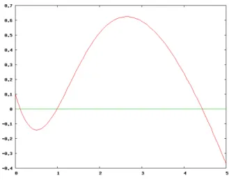
Hitherto we considered the case κ = 0. Let us consider the case κ > 0. Then the nonlinearity changes into the one like a bistable. We remark that the Gierer- Meinhardt (1.11) system possesses exactly one positive constant solution. Let us rewrite the system (1.11) simply as follows:

 



 

∂A

∂t

= ε

²

∆A + f (A, H), A > 0 in Ω × (0, ∞ ), τ

^∂H_∂t

= D∆H + g(A, H), H > 0 in Ω × (0, ∞ ),

∂A

∂ν

=

^∂H_∂ν

= 0 on ∂Ω × (0, ∞ ).

(1.19) Here, f (A, H ) = − A +A

^p

/(H

^q

(1 + κA

^p

)) +σ

₀

and g(A, H) = − H +A

^r

/H

^s

. Let κ > 0 and σ

0

≥ 0 be small constants. Then we notice that 0 = f (A, H ) possesses three roots denoted by A = h

₋

(H ), h

0

(H), h

+

(H ) ( h

₋

(H) < h

0

(H ) < h

+

(H )) for each H ∈ I (see Figure 1.1), where I is a suitable open interval.

Figure 1.1: Graph of f (A, H ) with κ = 0.2, σ

0

= 0.1, H = 0.95.

For each H ∈ I, let us consider a scalar reaction-diﬀusion equation:

∂A

∂t = ε

²

∆A + f (A, H) in Ω, t > 0, (1.20)

(12)

under the homogeneous Neumann boundary condition. If Ω is a convex domain, then one easily knows that stable equilibrium solutions are A = h

₋

(H ) and A = h

+

(H) only, while the rest A = h

0

(H) is unstable. Therefore, we call (1.20) a scalar bistable reaction-diﬀusion equation. Set

J (H) =

∫

h+(H) h₋(H)

f (s, H )ds, H ∈ I.

Then we can see that there exists a unique H

^∗

∈ I such that J (H

^∗

) = 0, and J

⁰

(H

^∗

) 6 = 0. In the case H = H

^∗

, two stable solutions h

₋

(H ) and h

₊

(H ) are equi-stable. Therefore, one can expect an internal layer equilibrium solution to (1.20). Therefore, one can also expect an internal layer solution to (1.19).

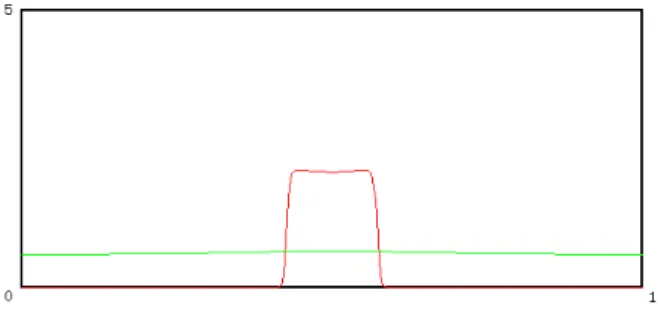
Indeed, when N = 1, for suﬃciently large D > 0 and suﬃciently small ε, M. Mimura et al. [61] showed that there exists internal multi-layer stationary solutions to (1.19) by using the singular perturbation method for more general nonlinear terms (see Figure 1.2). The stability was shown by Y. Nishiura and H. Fujii [82]. See also [88]. When also N ≥ 2 and Ω is a ball in R

^N

, the internal layer stationary solution exists (see [16] and [89]). From the bifurcation theory viewpoint, in [80], it is known that in the case N = 1, for suﬃciently large D, the bifurcating branch emanating from a constant solution to exist until it is connected to the internal layer solutions.

Figure 1.2: Internal layer. ε

²

= 5 × 10

⁻⁶

, D = 1.0, κ = 0.5, τ = 0.1. (p, q, r, s) = (2, 1, 2, 0)

For large amplitude stationary solutions, it seems that κ ≥ 0 must be small.

M. del Pino [15] showed the a priori estimate for a stationary solutions to (1.19) with (p, q, r, s) = (2, 1, 2, 0), κ, σ

0

∈ R

+

, such that

σ

0

≤ A ≤ 1

κσ

₀²

+ σ

0

, σ

²₀

≤ H ≤ ( 1 κσ

²₀

+ σ

0

)

2

. (1.21)

In general, if a stationary peak solution (A(x), H(x)) to the Gierer-Meinhardt

system exists, then the maximum value of A(x) on Ω becomes large in the order

of ε

⁻^N

as ε → 0. Hence, peak solutions has a large amplitude for suﬃciently

small ε. However, from the estimate (1.21), we see that such a large amplitude

stationary solutions does not exist provided κσ

²

is large.

(13)

1.2.5 Main results: weak saturation case

As we observed, stable peak solutions appear when κ = 0, and stable internal layer solutions appear when κ > 0. Now, does a peak stationary solution with large amplitude exist even if κ is positive? One of the answer is given under the weak saturation eﬀect. For the shadow system of the Gierer-Meinhardt system with (p, q, r, s) = (2, 1, 2, 0), κ > 0, σ

0

= 0,

 



 

∂A

∂t

= ε

²

∆A − A +

_ξ(1+κA^A² 2)

in Ω × (0, ∞ ), τ

^∂ξ_∂t

= − ξ +

_|_Ω¹_|

∫

Ω

A

²

dx in (0, ∞ ),

∂A

∂ν

= 0 on ∂Ω × (0, ∞ ),

(1.22)

J. Wei and M. Winter subjected the following condition:

(A.I) (weak saturation condition) κ > 0 depends on ε and there exists a limit lim

ε→0

ε

⁻^2N

κ = κ

0

∈ [0, ∞ ).

Under this condition, they showed the existence of the boundary single-peak stationary solution for suﬃciently small ε. When N = 1, the single-peak solution is stable provided τ is small. When N = 2, 3, it is stable provided κ

₀

and τ are small and the peak point is a nondegenerate local maximum point of the mean curvature function of the boundary. Although their result was the one for the shadow system, they give one of suﬃcient conditions to exist a peak solution in the case κ > 0.

Inspired from their work, we obtain a result on the existence of multi-peak stationary solutions to the full system (1.19) with κ > 0 and σ

0

= 0, for suﬃ- ciently small ε and large D when the domain Ω is axially symmetric. Moreover, we obtain a similar result for σ

0

6≡ 0 in the case (p, q, r, s) = (2, 1, 2, 0).

Theorem B. Let σ

₀

= 0. We assume (1.18). Suppose the weak saturation condition (A.I), and let κ

₀

be small enough. Let Ω be an axially-symmetric domain in R

^N

with respect to the x

_N

-axis. Let P

₁

, · · · , P

_2n

be the intersections of ∂Ω and the x

N

-axis. We choose points P

j₁

, · · · , P

j_m

from P

1

, · · · , P

2n

arbitrarily.

Then, for suﬃciently small ε and large D, there exist a boundary multi-peak stationary solution to (1.19), which concentrates at P

j₁

, · · · , P

j_m

.

Theorem C. Let σ

0

(x) be a nonnegative axially symmetric function on Ω of class C

^α

(Ω), α ∈ (0, 1). Let (p, q, r, s) = (2, 1, 2, 0) and 2 ≤ N ≤ 5. Suppose the same assumptions on κ and Ω, and let P

j1

, · · · , P

jm

be points, as in Theorem B. Then, for suﬃciently small ε and large D, there exist a boundary multi-peak stationary solution to (1.19), which concentrates at P

_j₁

, · · · , P

_j_m

.

The results above are on the stationary solutions to (1.19) near the shadow

system. Next, we consider the strong coupling case. In the case, we can show

that multi-peak stationary solutions exist under the same weak saturation con-

dition when N = 1, and we obtain the following theorem. Here, we remark that

the construction of solutions to the Gierer-Meinhardt system is more diﬃcult

in the strong coupling case than in the shadow system case.

(14)

Theorem D. Let N = 1, Ω = ( − 1, 1) and (p, q, r, s) = (2, 1, 2, 0). We assume that σ

0

is a nonnegative constant, and assume (A.I) for suﬃciently small κ

0

. Let D > 0 be given arbitrarily. Then, for suﬃciently small ε > 0, there exists a peak stationary solution to (1.19) which concentrates at the origin.

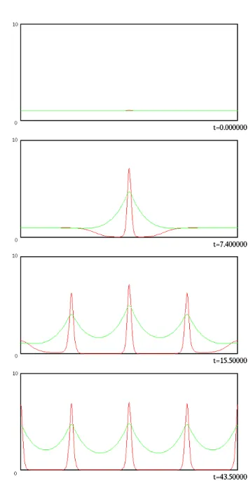
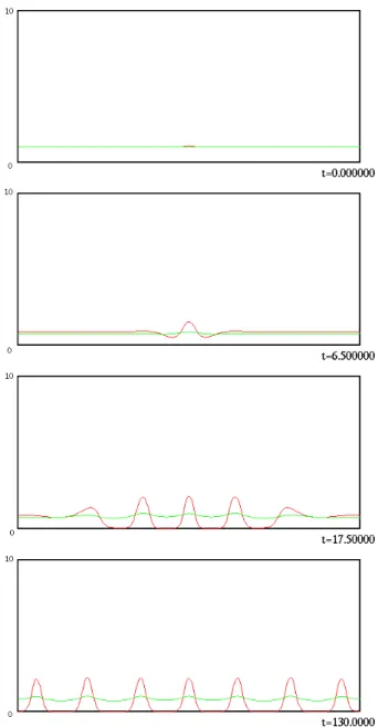
We note that, under the same situation as that in Theorem D, the existence of multi-peak solutions are ensured by reﬂections. See Figure 1.6 in the last section of this chapter, which is a numerical simulation of the one-dimensional Gierer-Meinhardt system. We see that multi-peak patterns appear if D is not so large.

1.2.6 Other topics for the Gierer-Meinhardt system and biological pattern formation

(N ≥ 2), it is known that (1.11) (κ = 0, σ

₀

= 0) has a stationary solution which con- centrate on a (N − 1)-dimensional sphere for ﬁnite D and suﬃciently small ε [79]. The Hopf bifurcations and Oscillatory instability of peak solutions for one- dimensional Gierer-meinhardt system were studied in [106]. Some interesting numerical simulations can be found in [86].

There is a characteristic solution, so-called a stripe pattern. A stripe pattern means that activator’s concentration localizes along the mid-line of the rectangular domain. K. Ikeda [34] rigorously proved that a stripe pattern is unstable when the saturation eﬀect is neglected. On the other hand, a lot of interesting numerical simulations were done by T. Kolokolnikov et al. [44]. They showed some patterns for the Gierer-Meinhardt system in a rectangular domain, stripes, wriggled stripes, self-replication of spots and so on. And they studied the stability and instability of the stripe pattern. In the process of collapse of a stripe pattern, several instabilities has been found, so-called, zigzag instability, breakup instability. However, it seems that a stripe pattern becomes stable provided the saturation eﬀect is enough. In fact, they showed a numerical simulation whereby a single stripe splits into two, with the two stripes undergoing a further splitting at later times, however, the stripe-shape does not collapse.

A Turing model has been suggested to explain the development of pigmen- tation patterns on certain species of growing angle-fish such as Pomacanthus semicirculantus where colored stripes are observed which change their number, size and orientation (see [45]). After this model was refined, adding effects such as cell growth and movement, also stripes of various thickness could be explained (see [85]). For reaction-diffusion systems on growing domains, which is a good model for the growth of organisms, see [13, 14, 55, 56].

From mathematical viewpoints, the uniqueness and the global existence of solutions to the initial-boundary value problem (1.11) are also interesting problems. For this direction, see [60, 57, 87, 96, 49, 37].

When κ = 0, the behavior of solutions to the following diﬀusionless system

(15)

was studied completely in [74]:

 



 

dA

dt

= − A +

_H^A^pq

, t > 0, τ

^dH_dt

= − H +

_H^A^rs

, t > 0, A(0) = A

0

, H(0) = H

0

.

(1.23)

Moreover, it was shown that (1.23) has a ﬁnite-time blow-up solution under some suitable condition.

1.3 Schnakenberg model

The Schnakenberg model [92] is a model equation of some chemical reaction on an activator and a substrate. The system is written as follows:

 

 



 

 

∂a

∂t

= ε

²

∆a − a + ha

²

, a > 0 in Ω × (0, ∞ ), τ

^∂h_∂t

= D∆h − ha

²

+ ρ, h > 0 in Ω × (0, ∞ ),

∂a

∂ν

=

^∂h_∂ν

= 0 on ∂Ω × (0, ∞ ), a(x, 0) = a

0

(x), h(x, 0) = h

0

(x) inΩ,

(1.24)

where ε, D > 0, τ > 0, k ≥ 0. a = a(x, t) and h = h(x, t) represent the concentrations of the activator and the substrate at x ∈ Ω and t ∈ (0, ∞ ), respectively. a

0

and h

0

are their initial data. ρ = ρ(x) represents the feed-rate of the substrate at x ∈ Ω. Let A and H be diﬀusive substances. Let P be a product. We consider the following chemical reaction processes:

2A + H → 3A, A → P.

Note that the product P is independent of the reaction between A and H . The Schnakenberg model describe these reaction processes. We note that the Gierer-Meinhardt system is a model of the activator and the inhibitor, and the inhibitor inhibits the reaction of the activator. Conversely, for the Schnakenberg model, the activator (A) is provided by substrate (H ), and the substrate decays.

Therefore, the feed of the substrate from outside is needed, and hence the feed rate ρ must be positive.

It is known that the Schnakenberg model also realizes the Turing instability. Namely, the spatial homogeneous state becomes unstable when ε

²

<< D.

Similarly to the Gierer-Meinhardt system, it is known that (1.24) admits multi-

peak stationary solutions. The existence and the stability of interior multi-peak

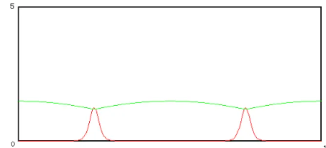
solutions have been studied in [36, 104] in the case N = 1 (see Figure 1.3). In

the case N = 2, interior multi-peak stationary solutions were constructed in

[116]. Moreover, the Schnakenberg model has been widely studied by analyt-

ical and numerical methods. We refer to [4] and the references therein. The

Schnakenberg model is a simple model of a chemical reaction. However, many

(16)

patterns observed experimentally can be computed, such as multi-spot forming hexagonal arrays, stripes and wiggled stripes (see [19]).

As in the case of the Gierer-Meinhardt system, we can consider the shadow system (which is a limit system of D → ∞ ) also for the Schnakenberg model, and the same analysis can be done. The steady-state shadow system can be written as follows: 

 

 

0 = ε

²

∆a − a + ξa

²

in Ω, 0 = ∫

Ω

( − ξa

²

+ ρ)dx,

∂a

∂ν

= 0 on ∂Ω.

(1.25)

By putting a(x) = ξ

⁻¹

u(x), the ﬁrst equation of (1.25) becomes

0 = ε

²

∆u − u + u

²

in Ω. (1.26) Hence, under the homogeneous Neumann boundary condition, we can show the multi-peak stationary solutions to (1.25) by the same consideration as in the case of the Gierer-Meinhardt system.

Figure 1.3: Peak solution. ε

²

= 0.0001, D = 0.01, ρ = 0.1, τ = 0.01.

1.3.1 Main result: Schnakenberg model with saturation

Now, we note that the Schnakenberg model can be regarded as a reaction- diﬀusion system of the resource-consumer type. A resource-consumer reaction- diﬀusion system is described as follows:

{

∂u

∂t

= d

_u

∆u + ωf(u, v) − g

₁

(u) in Ω × (0, ∞ ),

∂v

∂t

= d

v

∆v − f (u, v) + g

2

(v) in Ω × (0, ∞ ), (1.27)

under sutable boundary condition, where d

u

, d

v

> 0. u represents a concen-

tration of the resource, and v represents a density of the consumer. The term

f (u, v) means an interaction between the consumption and the production. The

constant ω means the conversion-rate from consumption to production. g

1

(u)

is a dissipation term, and g

2

(v) is a source term. From this viewpoint, it is not

(17)

unnatural to consider the saturation eﬀect to the Schnakenberg model which is written as follows:

 

 



 

 

∂a

∂t

= ε

²

∆a − a + h

_1+ka^a² 2

, a > 0 in Ω × (0, ∞ ), τ

^∂h_∂t

= D∆h − h

_1+ka^a² 2

+ ρ, h > 0 in Ω × (0, ∞ ),

∂a

∂ν

=

^∂h_∂ν

= 0 on ∂Ω × (0, ∞ ),

a(x, 0) = a

0

(x), h(x, 0) = h

0

(x) in Ω,

(1.28)

where k > 0. Because, the Schnakenberg model is originally a model of chemical reactions, such a model (1.28) with saturating growth has not be considered.

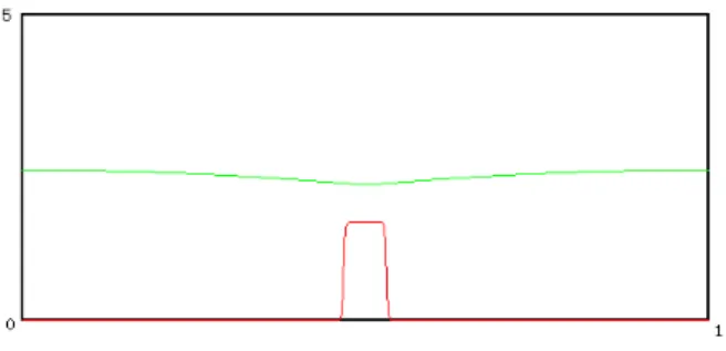
However, the author thinks it is interesting to consider the problem with saturation as in the case of the Gierer-Meinhardt system. Actually, we can ﬁnd that stationary internal layer solutions exists (see Figure 1.4). Indeed, by some transformation, the results in [61, 16, 89], which showed the existence of the internal layer solutions, can be applied (for the detail, see Section 5.3).

Figure 1.4: Internal layer. ε

²

= 10

⁻⁶

, D = 0.05, ρ = 0.1, κ = 1.0, τ = 0.01.

Similarly to the Gierer-Meinhardt system, under the weak saturation condition, we can construct multi-peak stationary solutions to (1.28) with k > 0 for suﬃciently small ε and large D in the case where Ω is an axially symmetric domain. The weak saturation condition for (1.28) is given as follows:

(A.II) k and ρ depend on ε and there exists a limit

ε

lim

→0

ε

⁻^2N

k ( ∫

Ω

ρ(x)dx )

2

= k

0

∈ [0, ∞ ).

In this case, the balance of k and ρ is important. We take P

_j₁

, · · · , P

_j_m

as in Theorem B. Then we can construct a multi-peak stationary solution to (1.28), and we obtain the following theorem:

Theorem E. Let 2 ≤ N ≤ 5, Ω be an axially symmetric domain, and ρ be an axially symmetric function of class C

^α

(Ω), α ∈ (0, 1), such that max

_Ω

ρ(x) > 0.

Suppose the condition (A.II) for suﬃciently small k

0

. Then, for suﬃciently

small ε and large D, there exists a multi-peak stationary solution to (1.28)

which concentrates at P

j₁

, · · · , P

j_m

.

(18)

1.4 Chemotaxis model

Chemotaxis. In the movement of biological individuals, microorganisms or cells sometimes move by responding to some chemical substance. This property is called a chemotaxis, and such a chemical substance is called a chemotactic substance. For example, Dictyostelium discoideum (D. discoideum) is a kind of microorganisms which show chemotaxis. D. discoideum is a single-celled organism like an amoeba. D. discoindeum moves at random and propagates when the feed of bacterium is enough. However, if the feed is not enough, then they secrete chemotactic substances each other, and move by recognizing the gradient of density, and form cellular aggregates.

Keller and Segel [39] proposed a mathematical model of chemotaxis. A simple form of the model can be described as follows:

 

 



 

 

∂P

∂t

= d

₁

∆P − ∇ · (P ∇ χ(W )) in Ω × (0, ∞ ),

∂W

∂t

= d

2

∆ + F (P, W ) in Ω × (0, ∞ ),

∂P

∂ν

=

^∂W_∂ν

= 0 on ∂Ω × (0, ∞ ),

P (x, 0) = P

0

(x), W(x, 0) = W

0

, x ∈ Ω,

(1.29)

where Ω is a bounded domain in R

^N

with smooth boundary. P = P (x, t) is the population density of individuals and W = W (x, t) is the concentration of chemotactic substance. The constants d

1

, d

2

> 0 are the diﬀusion constants of P and W , respectively. χ(W ) is called a sensitivity function of chemotaxis, and

∇ χ(W ) is the velocity of the direct movement of P due to chemotaxis. The function χ(W ) is generally assumed to be satisﬁed χ

⁰

(W ) ≥ 0 for W > 0. For example,

χ(W ) = p log(W ), pW, pW 1 + W ,

where p > 0 is a constant. And −∇ · (P ∇ χ(W )) stands for the movement of individuals. F (P, W) is the reaction term leading to production and degradation of W . The simplest form is F (P, W ) = − b

1

W + b

2

P with positive constants b

1

and b

2

.

Steady-state solutions. Under the concept of chemotaxis-induced instability, R. Schaaf [91] showed that there exist stable nonconstant equilibrium solutions, which indicate chemotactic aggregation of individuals. C.-S. Lin, W.- M. Ni and I. Takagi [53] treated the case χ(W ) = p log(W ) which had not been treated in [91], and they showed the existence of a large amplitude nonconstant stationary solution by using the Mountain Pass Theorem. More precisely, they showed the following:

(Result in [53]) Let F(P, W ) = − b

1

W + b

2

P and χ(W ) = p log(W ), p > 0.

Suppose that, p > d

1

if N = 1, 2, 1 < p/d

1

< (N + 2)/(N − 2) if N ≥ 3. Then there exists a large amplitude nonconstant stationary solution provided d

2

/b

1

is small enough.

After that, W.-M. Ni and I. Takagi [75] studied the shape of the least-energy

(19)

solution (which was given by the Mountain Pass Theorem), and showed the following:

(Result in [75]) If d

₂

/b

₁

is small enough, then the least-energy solution attains its maximum at exactly one point on the boundary ∂Ω (the point tends to the maximum point of the mean curvature function of the boundary), and the solution tends to 0 at the interior of the domain Ω as d

₂

/b

₁

→ 0.

Here, we recall that the works [53, 75] contributed also in the ﬁeld of the Gierer- Meinhardt system as a least-energy pattern. In the case N ≥ 3 and p/d

1

= (N + 2)/(N − 2), see [1, 9]. They assumed that Ω is an open ball, and studied the existence of radially symmetric stationary solutions. For general domain, the similar results as that in the case p/d

1

< (N + 2)/(N − 2) were given in [72]

with respect to the least-energy solution.

From the viewpoint of equation of evolution. In this viewpoint, the blow-up phenomenon is widely studied. Here, we say that u(x, t) blows up in ﬁnite time if there exists T ∈ (0, ∞ ) such that

lim sup

t→T

max

x∈Ω

u(x, t) = ∞ ,

and T is called a blow-up time. Additionally, we say that x

₀

∈ Ω is a blow-up point if there exists { (x

_n

, t

_n

) }

^∞n=1

⊂ Ω × (0, T ) such that x

_n

→ x

₀

, t

_n

→ T , u(x

_n

, t

_n

) → ∞ as n → ∞ . Let χ(W ) = pW and F (P, W ) = − b

₁

W + b

₂

P . V. Nanjundiah [70] conjectured that there exists a blow-up solution in ﬁnite time in the case N = 2. After that, S. Childress and J. K. Percus [11] conjectured the following:

1. In the case N = 1, blow-up solutions does not exists.

2. In the case N = 2, there exists a certain c > 0 such that, if ∫

Ω

P

0

(x)dx < c, then the blow-up does not arise, if ∫

Ω

P

0

(x)dx > c, then the blow-up in ﬁnite time may arise, and the blow-up solution tends to some delta function.

3. In the case N ≥ 3, independently of ∫

Ω

P

₀

(x)dx, the blow-up in ﬁnite time may arise.

It is known that the conjecture above is correct when N = 1. In the case N = 2, it is known that there exists a ﬁnite time blow-up solution provided Ω is a disk, and the blow-up point is the origin, and the blow-up solution is radially symmetric (see [30, 31]). Inversely, when Ω is a disk in R

²

, if there exists a ﬁnite time blow-up solution, then the blow-up point must be the origin only (see [68]).

Remark 1.1. Strictly speaking, the results in [30, 31, 68] above are the ones on the dimensionless system. The dimensionless system is given as follows:

In (1.29) with χ(W ) = pW (p > 0) and F (P, W ) = − b

1

W + b

2

P (b

1

, b

2

> 0),

(20)

transforming d

1

t 7→ t, and putting a = p

d

1

, τ = d

₁

d

2

, γ = b

₁

d

2

, α = b

₂

d

2

, we have the following dimensionless system:

 



 

∂P

∂t

= ∆P − a ∇ · (P ∇ W ) in Ω × (0, ∞ ), τ

^∂W_∂t

= ∆W − γW + αP in Ω × (0, ∞ ),

∂P

∂ν

=

^∂W_∂ν

= 0 on ∂Ω × (0, ∞ ).

(1.30)

This system can be treated more easily than original one.

Let N = 2. The unique existence of nonnegative local solution to (1.30) for the initial data (P

₀

, W

₀

) was given in [117]. For nonnegative classical solution (P (x, t), W (x, t)) to (1.30), the following properties are known (see [117, 69]):

1. Let T

_max

be a maximum existence time for (P, W). If P

₀

≥ 0, W

₀

≥ 0 and P

₀

6≡ 0, then

P (x, t), W (x, t) > 0, x ∈ Ω, 0 < t < T

max

. 2. If T

max

< ∞ , then

lim sup

t→Tmax

max

Ω

P (x, t) = ∞ , lim sup

t→Tmax

max

Ω

W (x, t) = ∞ .

3. If Ω is a disk in R

^N

, then P and W are radially symmetric provided P

0

and W

0

are radially symmetric.

The following results on the global existence of a solution were known (see [7, 21, 69]). Let Ω be a smooth bounded domain in R

²

. For nonnegative initial data (P

₀

, W

₀

), the following hold:

1. If ∫

Ω

P

₀

(x)dx < 4π/(aα), then the nonnegative global solution to (1.30) exists boundedly.

2. In particular, let Ω be a disk and ∫ P

0

, W

0

be radially symmetric. If

Ω

P

0

(x)dx < 8π/(aα), then the nonnegative global solution exists boundedly.

As we observed above, the chemotaxis model gave many interesting prob-

lems (existence of stationary spiky patterns, ﬁnite time blow-up solutions) to

mathematicians. For other related results and surveys, see [67, 93, 8, 94, 103,

54, 83, 95, 98, 97]. The works on the chemotaxis model which stem from Keller

and Segel are organized in [33].

(21)

1.4.1 Main results: chemotaxis model with saturation

Recently, the chemotaxis model with saturating growth has been studied, namely, such a model where the reaction term F(W, P ) in (1.29) includes a saturation eﬀect. In [83], the following case was treated

F (P, W ) = P W

1 + νW − µW + γ

_r

P 1 + P , where µ > 0, ν, γ

r

> 0. In [98], the case

F (P, W ) = − W + P W

1 + γW , γ > 0,

was treated, and the existence and the stability of the boundary single peak stationary solution were studied. Inspired from their works, we treat two cases as F (P, W ):

F

1

(P, W ) = − W + P W

^q

α + γW

^q

, (case A)

F

₂

(P, W ) = − W + P

1 + kP , (case B)

where q > 0, α, γ, k ≥ 0, and we assume χ(W ) = p log(W ) and 1 < p < ∞ if N = 1, 2; 1 < p < N + 2

N − 2 if N ≥ 3.

Let d

1

= 1, d

2

= ε

²

in (1.29). Then the system can be rewritten as follows:

 



 

∂P

∂t

= ∇ · (

P ∇ (log

_Φ(W^P ₎

) )

, (x, t) ∈ Ω × (0, ∞ ),

∂W

∂t

= ε

²

∆W + F (P, W ), (x, t) ∈ Ω × (0, ∞ ),

∂P

∂ν

=

^∂W_∂ν

= 0, (x, t) ∈ ∂Ω × (0, ∞ ),

(1.31)

with F (P, W ) being F

1

or F

2

. We assume that Ω is axially symmetric bounded domain in R

^N

with smooth boundary. Let P

_j₁

, · · · , P

_j_m

be points as in Theo- rems B. With respect to the saturation parameters, we assume the following:

(A.III) In the case A, α and γ depend on ε and there exists a limit

ε

lim

→0

ε

^N

(αγ

^q⁻¹

)

^1/q

= α

0

∈ [0, ∞ ).

(A.IV) In the case B, k depends on ε and there exists a limit

ε

lim

→0

ε

⁻^N

k = k

0

∈ [0, ∞ ).

Under these situations, we obtain the following results:

Theorem F. (case A) Suppose (A.III). For some α

1

∈ (0, ∞ ], if 0 ≤ α

0

< α

1

,

then, for suﬃciently small ε, there exists a multi-peak stationary solution to

(1.31) which concentrates at P

j₁

, · · · , P

j_m

.

(22)

It is a delicate problem whether the value α

1

above can be taken to be inﬁnite or ﬁnite. For the detail, see Chapter 4.

Theorem G. (case B) Suppose (A.IV). For each k

₀

∈ [0, ∞ ), if ε is suﬃ- ciently small, then there exists multi-peak stationary solution to (1.31) which concentrates at P

_j₁

, · · · , P

_j_m

.

1.5 About this thesis

In later chapters, we will study several partial diﬀerential systems stated before, the Gierer-Meinhardt system, the Schnakenberg model, the chemotaxis model.

For these models, we are mainly concerned with steady-state patterns, and we will study the existence of stationary peak solutions under the saturation eﬀect.

The existence of stationary peak solutions represents the point-condensation phenomena. We will study the relations between the point-condensation phenomena and the saturation eﬀect.

Motivation for our study

In the ﬁrst place, we will study the following equation in whole space:

{

∆w − w + f

δ

(w) = 0, w > 0 in R

^N

,

max

_RN

w = w(0), w(z) → 0 as | z | → ∞ , (1.32) where f

δ

(w) is a nonlinear term of w with a parameter δ. For example, f

δ

(w) = w

^p

/(1 + δw

^p

), p > 1. In the case where f

δ

(w) does not possess a parameter, for example f

_δ

(w) = w

^p

, the equation (1.32) has been studied widely. However, we will need to treat the problem (1.32) including a parameter. Let us show why we must treat such a problem, and why the solution to (1.32) will be needed for our analysis. We explain it using the Gierer-Meinhardt system in the case σ

₀

= 0, as an example. The steady-state Gierer-Meinhardt system is written as

follows: 

 

 

0 = ε

²

∆A − A +

_Hq(1+κA^A^p ^p)

, A > 0 in Ω, 0 = D∆H − H +

^A_H^r_s

, H > 0 in Ω,

∂A

∂ν

=

^∂H_∂ν

= 0 on ∂Ω.

(1.33)

Let P

1

, · · · , P

m

be m certain points on Ω. Let us assume that one wants to construct a multi-peak solution to (1.33) such that A(x) concentrates at the points P

1

, · · · , P

m

. However, it is hard to construct a solution (A, H ) to (1.33) directly. We ﬁrst construct a solution to the steady-state shadow system:

 



 

0 = ε

²

∆A − A +

_ξ_q_(1+κA^A^p _p₎

, A > 0 in Ω, 0 = − ξ +

_|_Ω¹_|_ξ_s

∫

Ω

A

^r

dx, ξ > 0,

∂A

∂ν

= 0 on ∂Ω.

(1.34)

(23)

For convenience, we set

γ := qr − (s + 1)(p − 1)

pq , γ

⁰

:= qr

p − 1 − (s + 1).

Note that γ, γ

⁰

> 0. If we put

A(x) = ξ

^q/(p⁻¹⁾

u(x), (1.35) and substitute this into the shadow system (1.34), then we have the following equation for (u, ξ):

 

 



 

 

ε

²

∆u − u + u

^p

1 + κξ

^pq/(p⁻¹⁾

u

^p

= 0 in Ω, ξ

^γ⁰

= ∫ | Ω |

Ω

u

^r

(x)dx ,

∂u

∂ν = 0 on ∂Ω.

(1.36)

Note that ξ includes the integral of u

^r

. Hence, we remark that this system can be regarded as a nonlocal scalar equation. Now, we put δ = κξ

^pq/(p⁻¹⁾

, then problem (1.36) is reduced to the problem: ﬁnd the pair of u and δ satisfying

 

 

 

 



ε

²

∆u − u + u

^p

1 + δu

^p

= 0 in Ω, δ

^γ

∫

Ω

u

^r

(x)dx = κ

^γ

| Ω | ,

∂u

∂ν = 0 on ∂Ω.

(1.37)

If we can ﬁnd a pair of (u, δ) satisfying (1.37), then the solution to (1.36) is also obtained. For the purpose, we ﬁrst consider the single Neumann problem with parameters ε and δ:

{

ε

²

∆u − u + f

δ

(u) = 0 in Ω,

∂u

∂ν

= 0 on ∂Ω, (1.38)

f

δ

(u) = u

^p

1 + δu

^p

. (1.39)

Then, our construction of a peak solution to (1.33) is organized as follows:

Step 1. We construct a solution to (1.38) peaked at P

₁

, · · · , P

_m

, denoted by u

_δ

(x; ε), for suﬃciently small ε > 0.

Step 2. We ﬁnd δ = δ

_ε

satisfying the second equation of (1.37) with u = u

_δ

( · , ε).

Step 3. By putting

A

_ε

(x) = ξ

^q/(p_ε ⁻¹⁾

u

_δ_ε

(x; ε), ξ

_ε

=

( ∫ | Ω |

Ω

u

^r_δ

ε

(x; ε)dx )

1/γ⁰

,

we obtain a one-parameter family of solution (A

ε

, ξ

ε

) to the shadow system

(1.34).

Point-condensation phenomena and saturation eﬀect for the Gierer-Meinhardt system ギーラー・マインハルト系における