FastComputationwithE ﬃ cientObjectDataDistributionforLarge-ScaleHologramGenerationonaMulti-GPUCluster PAPER

(1)

PAPER

Fast Computation with E ﬃ cient Object Data Distribution for Large-Scale Hologram Generation on a Multi-GPU Cluster

Takanobu BABA^†^a),Fellow, Shinpei WATANABE^††^b), Boaz JESSIE JACKIN^†††^c),Nonmembers, Kanemitsu OOTSU^††††^d), Takeshi OHKAWA^††††^e), Takashi YOKOTA^††††^f),Members, Yoshio HAYASAKI^†^g), andToyohiko YATAGAI^†^h),Nonmembers

SUMMARY The 3D holographic display has long been expected as a future human interface as it does not require users to wear special devices.

However, its heavy computation requirement prevents the realization of such displays. A recent study says that objects and holograms with several giga-pixels should be processed in real time for the realization of high resolution and wide view angle. To this problem, first, we have adapted a conventional FFT algorithm to a GPU cluster environment in order to avoid heavy inter-node communications. Then, we have applied several single-node and multi-node optimization and parallelization techniques.

The single-node optimizations include a change of the way of object decomposition, reduction of data transfer between the CPU and GPU, kernel integration, stream processing, and utilization of multiple GPUs within a node. The multi-node optimizations include distribution methods of object data from host node to the other nodes. Experimental results show that intra-node optimizations attain 11.52 times speed-up from the original single node code. Further, multi-node optimizations using 8 nodes, 2 GPUs per node, attain an execution time of 4.28 sec for generating a 1.6 giga-pixel hologram from a 3.2 giga-pixel object. It means a 237.92 times speed-up of the sequential processing by CPU and 41.78 times speed-up of multi-threaded execution on multicore-CPU, using a conventional FFT- based algorithm.

key words: computer generated holography, large-scale CGH, GPU clus- ter

1. Introduction

The 3D holographic display has long been expected as a future human interface as it does not require users to wear special devices[1]. In display systems, the computer receives 3D object data, computes wave propagation from each object point to each hologram point as well as the interference with a reference laser beam and stores the whole result

Manuscript received October 12, 2018.

Manuscript revised February 1, 2019.

Manuscript publicized March 29, 2019.

†The authors are with Center for Optical Research and Educa- tion, Utsunomiya University, Utsunomiya-shi, 321–8585 Japan.

††The author is with Acs Co., Ltd., Ashikaga-shi, 326–0333 Japan.

†††The author is with National Institute of Information and Com- munications Technology, Koganei-shi, 184–8795 Japan.

††††The authors are with Department of Information Systems Sci- ence, Graduate School of Engineering, Utsunomiya University, Utsunomiya-shi, 321–8585 Japan.

a) E-mail: [email protected] b) E-mail: [email protected] c) E-mail: [email protected]

d) E-mail: [email protected] e) E-mail: [email protected] f) E-mail: [email protected] g) E-mail: [email protected] h) E-mail: [email protected]

DOI: 10.1587/transinf.2018EDP7346

to a SLM (Spatial Light Modulator). By applying a reference laser illumination to the SLM, the diﬀraction pattern regenerates the object wave and the user can see the reconstructed 3D object as if it exists at the original position. This process is well-known as computer generated holography (CGH)[2],[3].

One of the largest issues for realizing such display systems is their requirement for a huge number of computa- tions. The computation cost of wave propagation from N object points toNhologram points becomesO(N²)[9]. In order to solve this problem, a wide variety of approaches have been taken. To accelerate the calculation of point-to- point wave propagation, a table-lookup method is used to evaluate trigonometric functions[4],[16]. Architectural approaches include the development of special-purpose computers using large-scale FPGA chips[10],[11]and the utilization of GPU and GPU clusters[9],[12]–[15],[18],[25].

In order to reduce the large cost of point-to-point calculation, FFT-based methods are used to improve the order of computation fromO(N²) toO(NlogN)[17]. However, for the size of the objects and holograms these projects treat, the processing time for one frame becomes hundreds to even thousands of seconds[12],[26].

On the other hand, the capability of 14.7 giga pixel object display is required for the human eyes’ recognition capability[7]. Further, a 4.5 gigapixel SLM is needed to realize view angles of 20 degree for 7 inch objects[8]. Thus, the giga-pixel order is required to realize the high resolution and wide view angle needed to match the human interface.

If we treat, for example, 4 giga-pixels, each pixel requires 8B as a complex number representation and a total of 32 GB of memory space is required to store just the object data. We need additional memory space for the output hologram and working space. The global memory size of current GPUs is far behind these requirements[28]. Thus, if we want to utilize the parallel computation capability of GPU clusters as well as the low computation cost of FFT based methods, we need to decompose the input object into multiple sub-objects and apply distributed FFT algorithms to them. In this case, we encounter a further problem that the distributed FFT algorithms require a lot of node-to-node data transfer for realizing butterfly operations[18].

To this problem, we have been working on a distributed algorithm, called a decomposition method, for generating 2D Fourier holograms[5]and 3D Fresnel holograms[6]. In order to estimate the performance of the method, we per- Copyright c⃝2019 The Institute of Electronics, Information and Communication Engineers

(2)

formed a simulation. In this simulation, as we could not use GPU-clusters, we first obtained computation time on a single multi-GPU node without application-oriented optimizations and inserted the time to the CPU-cluster program by using the nano-sleep library function. The simulation results were used for showing the advantage of our decomposition method over conventional methods. In parallel with the simulation, we have also developed a real GPU cluster using 8 nodes of multi-GPU machines, implemented the decomposition method for 3D Fresnel hologram generation on the cluster and applied application-oriented optimizations[19]–

[21]. Thus, the major diﬀerences of this research from[6]

are that this research utilizes a real multi-GPU cluster and applies various application-oriented, single-node and multi- node optimizations to verify their eﬀectiveness.

Aiming for the ultimate goal of realizing 3D holographic display with high-resolution and wide view angle properties in real time, this research revises the results of [19],[20]and[21]and shows how we resolve the diﬃculties of large-scale CGH generation on a multi-GPU cluster by adapting the FFT-based algorithm to the clusters’ environment and how to apply application-oriented optimizations under the multicore-CPU and multi-GPU combined heterogeneous architecture.

This paper is organized as follows. Section 2 describes the basic concept of the conventional FFT-based CGH generation and the object decomposition method. Sections 3 and 4 describe the application of optimizations within single node and multiple nodes, respectively. Section 5 shows experimental results using a multi-GPU cluster. Section 6 concludes the paper.

2. Algorithm Adaptation for GPU Cluster Implemen- tation

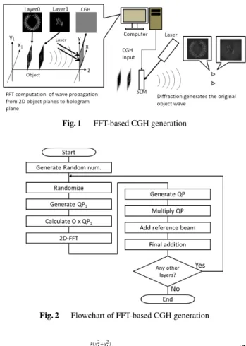
Figure 1 shows the process of 3D image reconstruction using conventional FFT-based methods. Notice that a 3D object is represented as multiple 2D planes, calledobject lay- ers, in order to apply 2D-FFT operations. In the figure an input object consists of two layers placed at diﬀerent positions. Firstly, the wave propagation from these multiple object layers to the hologram plane is computed by applying 2D-FFT operations; then, the interference with the reference laser beam is added to make hologram data, calledinterfer- ence fringes; then, this hologram data is transferred to the SLM; finally, by illuminating the SLM with the reference laser light the diﬀraction regenerates the object wave from the 3D object. This regenerated wave enables the viewer to see as if the original object exists at the original position.

Equations (1) to (3) below express the wave propagation computation from an object layerO(x₁, y1) to the hologram planeH(x, y).

H(x, y)=QP(x, y)×FFTN×N[(O(x1, y1)

×QP1(x1, y1))] (1)

QP(x, y)=e^j^k(x

2+y2 )

2z (2)

Fig. 1 FFT-based CGH generation

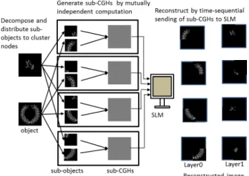
Fig. 2 Flowchart of FFT-based CGH generation

QP1(x1, y1)=e^j

k(x2 1+y2

1)

2z (3)

In these expressions,Hrepresents a hologram plane,x andyrepresent the hologram plane’s horizontal and vertical coordinates, respectively, Ois the two-dimensionalobject layer,x₁andy1 are the object’s horizontal and vertical coordinates,zrepresents the distance from the object layer to the recording hologram plane,Nis the number of pixels on one dimension of the object, andkis the value of 2πdivided by the wavelength of light (λ).

Figure 2 shows the flow of conventional FFT-based 3D Fresnel hologram computation. The five steps from “Gen- erateQP₁” to “Multiply QP” realize Eq. (1). That is, “Gen- erate QP1” and “CalculateO×QP1” computeO(x1, y1)× QP₁(x₁, y1). The next step “2D-FFT” realizesFFT_N_×_N. The next two steps of “GenerateQP” and “Multiply QP” realize multiplication by Eq. (2). Notice that the first two steps of

“Generate Random num.” and “Randomize” are inserted as an optical convention so that light from all parts of the object can spread over the hologram plane[22]. The step “Add reference beam” implements the interference with the reference light. The “Final addition” accumulates all the results for diﬀerent layers.

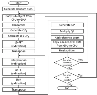
Figure 3 shows the process of hologram computation and 3D image reconstruction using the object decomposition method[5]. In the figure, the input object consists of two 2D object layers, a pigeon and an olive. Each object layer is first decomposed intosub-objects; in the figure, we assume the use of 4 nodes and decompose the object layer into 4 sub-objects; then the three operations of interpolation,

(3)

Fig. 3 CGH generation and its display mechanism of object decomposition method

FFT, and shift are applied to each sub-object to produce a hologram, called asub-CGH; by adding two sub-CGHs for sub-objects of diﬀerent layers we can obtain the final sub- CGH; and by illuminating this final sub-CGH the original sub-objects are reconstructed at their original positions.In- terpolationis necessary to keep the original bandwidth and make the object segment reconstructed successfully. Ashift operation is necessary for reconstruction at the original position of the object segment. Without this shift, all the object segments are reconstructed at the upper-left corner. Theo- retically, if we add up all the sub-CGHs, we can obtain the same results with those obtained by the conventional FFT- based method[17]. However, in order to save this addition time, we suppose the display system which switches its input from among the generated, multiple sub-CGHs. This enables us to reconstruct the original 3D object by time sequential reconstruction of sub-objects. We have proved that if the time sequential reconstruction is performed at an appropriate speed, the whole original 3D image is per- ceived[5],[6].

Notice that the boxes in Fig. 3 indicate that after the original object is decomposed and distributed to parallel processing units, the computation from sub-object to sub- CGH and reconstruction can be performed in a mutually independent manner.

For the theoretical background and optical verification of the decomposition method as well as the preliminary results of its application to the Fourier and Fresnel hologram generation, see[5]and[6], respectively.

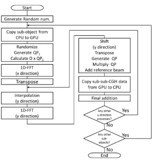
Figure 4 shows the basic flow of the decomposition method that generates each sub-CGH from each sub-object.

In the figure, the interpolation, 1D-FFT and shift operations are applied in thex- andy-directions, sequentially. This process is repeated for diﬀerent object layers and the results are accumulated by the final addition. Notice that the functions from “MemcpyHtoD” to “MemcpyDtoH” are executed in the GPUs. Thus, the time-consuming “Add reference beam”

should be included in these functions.

At first, we have implemented this flow on a single-

Fig. 4 Flowchart of the decomposition method

Fig. 5 Generation process from sub-object to sub-CGH

node with multiple GPUs as the base program of further optimizations and parallelization. Considering the limited global memory size of each GPU, we have tried to oﬀ-load the sub-object to sub-CGH generation, the most heavy computation part, to the GPUs. The CPU controls the global flow and does memory intensive work, i.e. keeping the whole object and the generated sub-CGH.

Figure 5 shows an illustration of the sub-CGH generation process by the loop iterations in the flowchart. At the first iteration, the application of the x andydirection operations to each sub-object produces the same size of partial sub-CGH, calledsub-sub-CGHdata. A GPU performs this part of the computationKtimes, whereKrepresents the number of decompositions, and sends the results to the CPU.

Then, the CPU adds the sub-sub-CGH data to the predeter- mined area, as shown in Fig.5(a). In the figure, jis used as an index for counting loop iterations up to the number of decompositions, i.e.,K.

By filling up the sub-CGH area in CPU memory by

(4)

four times of sub-sub-CGH data, sent from GPU, the sub- CGH is completed. Notice that the number of loop iterations reflects the number of decompositions. Thex- andydirection operations should be repeated by the number ofx- andy-direction decompositions, respectively. For example, if the input object is decomposed like Fig. 3 the numbers of x- andy-direction iterations become 2 and 2, respectively, and a total of 4 sub-sub-CGH data generation processes are performed.

This means that the increase of the number of decomposition increases the number of loop iterations and thus the total computation cost. Therefore, from the view point of computation cost, a small number of decompositions is good. On the other hand, from the view point of global memory size, a large number of decompositions is good as it makes the sub-object size small. Thus, in general, we should select the number of decompositions as a tradeoﬀpoint of these two aspects.

Comparing with the conventional method, the decomposition method requires less communication as the computation processes from sub-objects to sub-CGHs are mutually data-independent. Thus, once the original object is decomposed into sub-objects and sent to computing nodes, no node-to-node communications are necessary at all. No- tice the final reconstructions are also mutually independent.

Another important aspect of the decomposition method is that it requires much less GPU memory space, since just the decomposed sub-object and the corresponding partial sub- CGH data are treated in the GPU. This is critical for generating gigapixel hologram using a limited global memory space of GPU.

However, we should be careful about the following two points: first, the decomposition method increases the amount of computation for interpolation and space-shift;

second, the sub-CGH generated from the sub-object requires the same size of memory space as the whole CGH.

Thus, the key issues of object decomposition method implementation on GPU clusters are to determine: i) whether the additional computation cost for the interpolation and shift operations is paid back by less communication and by the deletion of the addition of sub-CGHs, and ii) whether the sub-sub-CGH data is generated within a limited global memory space of GPU and appropriately stored back to the host CPU to make sub-CGH used for the reconstruction. Our eﬀort of optimizations and parallelization (Sects. 3 and 4) and the experimental results (Sect. 5) will answer these issues.

3. Single-Node, Multi-GPU Optimizations

This section describes the optimizations and parallelization within a single node with multiple GPUs.

3.1 Changing Distributed Accesses to Contiguous Ones (Optimization 1)

When we send data from the CPU to a GPU, the data transfer

Fig. 6 Change from two-dimensional decomposition to one-dimensional one

Fig. 7 Flowchart after optimization 1

is performed by the cudaMemcpy function, which requires the input data to be on a contiguous address space.

At first, we decompose the input object plane into x- andy-directions like shown in Fig. 6 (a). In this case, we need to rearrange the data so that the selected parts become contiguous in memory before transferring from CPU to GPU.

We have improved the way of decomposition by changing toy-direction only decomposition, as shown in Fig. 6(b).

This makes the decomposed areas contiguous in memory and we can transfer the data without rearrangement.

Figure 7 shows the flow after this optimization. By comparing this flow with the original flow of Fig. 4, we can understand that, in the original flow, the combination of the x- andy-direction operations is repeatedly executed. How- ever, in Fig. 5, once the x-direction operation is executed, the resulting data in local memory can be utilized repeatedly by the followingy-direction operations. This not only reduces the number of kernel executions for x-direction operations but also enables the passing of temporal computation results from ax-direction computation to ay-direction one through high-speed local memory.

Notice that in the original way of decomposition the number of decompositions should beN²whereN=1,2, . . ..

(5)

Fig. 8 Reduction of data size transferred between CPU and GPU

However, this change of the way of decomposition alters the number to justNand thus makes it easier to adjust the sub- object size to the limitation of a GPU’s memory size. In our implementation, for the ease of coding,N is selected as 2ⁿ wheren=1,2, . . ..

3.2 Reduction of Data Transfer Amount between CPU and GPU (Optimization 2)

As the data transfer time between CPU and GPU adds to the computation time, the GPU’s fast computation may be im- paired by the slow transfer time. Thus, we should be careful about the contents of the transfer.

Our CGH generation program uses cufft, a CUDA library, for the FFT computation[23]. It requires cufftCom- plex as its input array. The cufftComplex consists of a real part and an imaginary part, and each part requires 4B memory space for storing floating point data. Thus, in our original program, both CPU-to-GPU input transfer and GPU-to- CPU output transfer use an 8B cufftComplex type.

However, the use of this data type is redundant. A pixel of the input object uses just one byte of the real part. This can be replaced with 8-bit unsigned integers. In a similar manner, the output from GPU only uses a 4B real part and can be replaced with a floating point number.

Figure 8 shows this change schematically. The reduction of the data size shortens the data transfers from CPU to GPU and from GPU to CPU. However, the GPU must perform the additional tasks of extension from the input 8-bit to 8-byte complex type and reduction from 8-byte complex type to 4-byte real type. Experimental results are expected to clarify the total eﬀect.

3.3 Kernel Integration and Utilization of High-Speed Memory (Optimization 3)

Usually, a GPU has thousands of execution cores for arith- metic and logical operations[24]. In order to utilize their computing power eﬀectively, it is critical to smoothly pro- vide them data to be processed. For this purpose, a GPU has a hierarchically structured memory system of register file, local memory, cache memory (usually multi-level), and global memory. The input data to a GPU is first sent to the global memory. When a kernel starts its execution, it reads data from the global memory to a higher level memory and

Fig. 9 Kernel integration

tries to keep the data at the higher level until the end of the execution. At the end of the execution, the results should be saved to global memory to pass them to the succeeding kernel. Then the succeeding kernel reads the data again into higher level memory to perform its operation. The problem here is the large overhead of this write-back and read-out cost of global memory, the slowest memory in the hierar- chy. We cannot overlook that these write-back and read-out operations also lose the locality of references.

In order to solve this problem, we have tried to inte- grate kernel functions into one kernel function as much as possible. Figure 9 shows the integrations of the three kernels from “Randomize” to “Calcurate O×QP1” and the five kernels from “Shift” to “Add reference beam”. These kernels are called separately from the CPU in Fig. 7. Be- fore the integration, each kernel reads all the pixels from global memory, applies each computation and stores the results back to global memory. After the integration, the three kernel functions are combined into one kernel function. This kernel function reads a part of the pixels from global memory, applies the three operations to them, i.e. Shift, Trans- pose and Multiply QP, and stores the partial results back to global memory, repeatedly, until all the pixels are processed.

By this integration, we can utilize higher-level memories, such as registers and shared memory, for inter-kernel data passing. The integration also reduces the number of kernel function calls and, thus, reduces the cost for GPU control.

3.4 Stream Processing of GPU Calculations and Transfer of the Result (Optimization 4)

As shown in Fig. 5, the sub-CGH, generated from the sub- object, becomes the same size as the final CGH. Thus, we need to send the partial results, i.e., sub-sub-CGH data, back to the CPU repeatedly to save the limited memory space of the GPU. Fortunately, the generation process can be divided

(6)

Fig. 10 Design of stream processing between GPU and CPU

intoKmutually data-independent operations whereKrep- resents the number of decompositions. Thus, we repeat the processKtimes.

We have utilized stream processing to treat these computation and communication pairs eﬃciently, as shown in Fig. 10. That is, first, the pair of the partial result calculations in the GPU, represented as A and B, are executed.

Then, the results are transferred from the GPU to the CPU by sub-CGH data transfer operation, represented as C. Fi- nally, the final addition operation, D, is executed in CPU.

The pipelining of these operations should take into ac- count the following conditions. The first pair of calculations should be serial as B inputs the output of A. The transfer from GPU to CPU should wait for the completion of B in the GPU. The calculation at A should wait for the completion of B of the preceding pipeline as they share the same buﬀer memory.

3.5 Utilization of Multiple GPUs under the Control of a Multicore CPU (Optimization 5)

If multiple GPUs are available in a single node, we may utilize their parallel processing capability. In this case, it is de- sirable to assign them mutually data-independent processing so that they can execute in parallel.

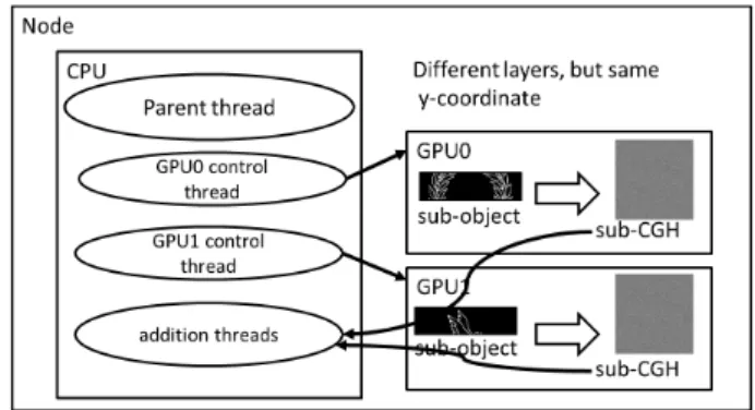
In the CGH generation, if we assign sub-objects of dif- ferent layers to the multiple GPUs, the generation process becomes mutually independent. In order to control these parallel operations in multiple GPUs, we use multithreading in the CPU. One thread controls one GPU, by specifying the GPU using cudaSetDevice[23].

One important issue for utilizing the multiple GPUs is how the CPU receives the results of the computation from them and, if necessary, does some reduction operations on the results. In our decomposition model, the reduction operation is the addition of sub-CGHs generated from diﬀer- ent object layers. as shown in Fig. 11. We considered three methods to treat this issue: (i) providing disjoint areas for diﬀerent GPUs, (ii) using “lock” to prevent the other threads from modifying the same area, and (iii) using a synchroniza- tion mechanism to avoid allowing the two threads to handle the shared data area simultaneously. We performed preliminary evaluation of these methods and found that (iii) attains the best performance[19]. Thus, we use this method for our

Fig. 11 Multi-thread controlled multi-GPU

experiments, as described in Sect. 5.

4. Multi-Node Optimizations

The major principle of the decomposition method is to save communication cost by avoiding the frequent data transfers required for 2D-FFT operations. Following this principle, we assign sub-objects with the same x- and y-coordinate values but with diﬀerent layers to a single node. This as- signment avoids unnecessary data transfers during the computation.

One inevitable data transfer operation occurs when the host node distributes sub-objects of diﬀerent layers to the other nodes. We must consider that the input object is given in a compressed image file, such as JPEG and PNG. The object in the compressed format can not be decomposed and used for further computation and we need to decompress it before decomposition. Thus, there are two possibilities.

The first method is to decompress the input object to bitmap, i.e., one pixel to 8-bit unsigned integer, on the host node, decompose the decompressed object into sub-objects, and transfer each sub-object to an appropriate node. In this method, the transfer amount, i.e., the sub-object size, is determined statically. Further, it should be smaller than the size of the original compressed object. Figure 12 shows how the input object is decompressed and decomposed into sub-objects in the host node, Node 0, and sent to the other nodes for sub-CGH generation. The decompressed and decomposed sub-objects are sent by MPIsendandrecvpair operations, sequentially[27].

The second method is that the host node first distributes the compressed whole object to all the other nodes, as shown in Fig. 13. Then, each node decompresses the input object and extracts the sub-object to be processed in the node. In this method, the data size of the compressed object is dy- namically determined. Thus, the size should be distributed first from the host to the other nodes so that they can allo- cate necessary memory space for storing input compressed object. The MPIbroadcastis used to distribute the compressed whole object. Each node needs to perform decom- pression separately. For the details of the sending procedure by using MPI, see[19].

In the following section, we will show the performance

(7)

Fig. 12 Decompress-and-unicast method

Fig. 13 Multicast-and-decompress method

results of these two methods.

5. Experimental Results

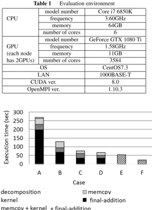
We have performed experiments in order to verify the eﬀec- tiveness of the optimizations. The execution environment is summarized in Table 1. Simply speaking, it is 1000BASE-T connected 8 node GPU cluster with each node containing two GPUs. Many similar projects use a high-speed network, such as Infiniband, to treat this kind of large-scale bandwidth intensive task without locality[18],[25]. Unlike them, we use a low cost gigabit Ethernet. We use C to describe CPU code, Pthreads to describe multithreading for optimization 5, MPI Ver. 1.10.3 to describe the internode communication, and CUDA version 8.0 to describe the GPU code.

The input object consists of a pair of PNG files (40K×

Table 1 Evaluation environment model number Core i7 6850K

CPU frequency 3.60GHz

memory 64GB

number of cores 6

model number GeForce GTX 1080 Ti

GPU frequency 1.58GHz

(each node memory 11GB

has 2GPUs) number of cores 3584

OS CentOS7.3

LAN 1000BASE-T

CUDA ver. 8.0

OpenMPI ver. 1.10.3

Fig. 14 Single-node results

40Kfor each) and the total data size is 141.3MB. They are decompressed into two bitmap files (1.6GB for each) by using an OpenCV function. Thus, the total size of the input object is 3.2 giga-pixels. The hologram size is 1.6 giga- pixels.

Following the discussion in Sect. 2, the number of decompositions is determined to be 8 as a trade-oﬀbetween the decomposed object size and computation cost.

Our first experiment is to apply the optimizations 1 through 5 to clarify their eﬀect in a single node. Throughout the experiment the number of decompositions is fixed at not 8, as determined above, but 16. The reason is that the number should be 2²ⁿbefore optimization 1, as noted in 3.1, and we must use the same value consistently during single-node optimizations. Thus, the host CPU sends a total of 32 (= (number o f decomposition)×(number o f layers)=16×2) sub-objects to the GPUs to process all of them.

Figure 14 shows the execution time results where the time of each bar is decomposed into the times for decomposition, memory copy (memcpy), kernel, and the final addition. The decomposition and final addition are done by the CPU. Memory copy includes both CPU-to-GPU and GPU- to-CPU transfers. The kernel processes 32 sub-objects and the kernel time includes the kernel-call time.

The barArepresents the starting point of our optimization. Conventional optimizations, such as an appropriate definition of grid and blocks, coalescing access of global memory, and eﬃcient use of local memory, have already been applied.

(8)

The bar B shows the eﬀect of optimization 1. The change in decomposition method eliminates the decomposition time, shown as a very small white box at the top of barA. It also reduces the kernel time as the results of the x₁ direction processing is repetitively utilized as described in 3.1. Notice that the eﬀect of results output as contiguous memory space also shortens the final addition time of CPU.

The barCshows the eﬀect of optimization 2. The results show that the increased kernel time reduces memory copy time. Changing from a complex data type to a real one also reduces the time for the final addition on the CPU.

The barDshows the eﬀect of optimization 3. The integration of kernels naturally reduces the kernel time.

As to the barsEandF, we cannot simply decompose the execution time as the optimizations realize parallel operations between computation and communication (optimization 4) and between multiple GPUs (optimization 5).

The barEshows the eﬀect of stream processing. The measured time shows improvement, but not as much as we initially expected. The reason is twofold: first, in order to save the memory space of GPU, we did not utilize double buﬀering between the four operations, and second, the execution times of four pipe-stages are imbalanced (the execution time ratio of the pipe-stages A, B, C and D in Fig. 10 was 1:1:2:4) and the fourth stage of addition by CPU becomes the bottleneck.

The barFrepresents the eﬀect of optimization 5. Using two GPUs nearly halves the time forE.

Eventually,Fattains a 11.52 times speed-up fromA.

Figure 15 shows the execution times of the CPU and the GPU cluster, while changing the number of cluster nodes.

The left-most bar represents the sequential processing time by the CPU, following the flow of Fig. 2, i.e. a conventional FFT-based algorithm. The CPU uses just the CPU part of Table 1. The sequential code is written in C and the 2D-FFT is realized by the FFTW 3.3.2 library. We obtain this time as the baseline performance. Thus, we intention-

Fig. 15 Multi-node results

ally do not utilize CPU parallelism, such as multicore multithreading and SIMD extensions. The results show 1018.32 seconds of processing time.

For the experiment using the 8 node GPU cluster, we fixed the number of decomposition at 8. This is based on the discussion in Sect. 2.

For the next bar of 1 node we use one node of the GPU cluster defined in Table 1. From 2 nodes to 8 nodes, we applied the multi-node optimizations described in Sect. 4.

The bars for (a) and (b) show the execution time for the decompress-and-unicast method and multicast-and-decompress one, respectively. Each bar is decomposed into CGH generation time and transfer one.

From the results we understand that broadcasting compressed object is much faster than sequential unicasting of decompressed sub-objects. The reason is as follows:

the broadcasting transfers the same data to all nodes and thus the total transfer amount of the method (b), i.e., compressed object, became 141.3 MB (i.e., size of 2 PNG files); on the other hand, that of method (a), i.e., decompressed and decomposed data for 8 nodes, uses multiple unicasting and its total transfer amount became 2.8 GB (= (size o f decompressed and decomposed ob ject)× (number o f nodes−1) = 400MB×7). Thus, the method (a) is even slower than the execution time by a single node.

From the viewpoint of scalability, the increase of nodes decreases the generation time but at the same time increases the transfer time. Even in method (b), the transfer time slightly increases. These results indicate that the bottleneck of the current system exists in the transfer time.

The rightmost bar indicates that 8 nodes cluster attains the execution time of 4.28 sec, which means 237.92 times speed-up of the sequential processing on CPU.

Further, for fair comparison with a CPU without GPUs, we have performed an experiment of multi-threading on a multicore-CPU using OpenMP. The program has been com- piled by gcc ver.4.8.5(CentOS 7’s default compiler) with optimization option -O3. As the multi-node implementation is slower than the single node one due to its heavy node-to- node communication costs and low communication speed of 1000BASE-T network, we show the single CPU results in Fig. 16.

Fig. 16 CPU-only results by multithreading

(9)

The results show that the case for 12 threads attains the shortest execution time of 178.81 sec. This means that our results attain 41.78 times better performance than that for a multicore-CPU.

6. Conclusion

We have described our research results for overcoming the diﬃculty of large-scale CGH generation on a multi-GPU cluster. Our eﬀorts include algorithm adaptation for a multi- GPU cluster and both intra- and inter-node optimizations of the code for multicore CPU and multi-GPU combined heterogeneous node architecture.

The intra-node optimizations attain an 11.52 times speed-up from the original single node code. The extreme results, using our 8 nodes 2-GPU architecture, show a 4.28 sec execution time for generating a 1.6 giga-pixel hologram.

This is 237.92 times faster than the sequential processing by CPU using a conventional FFT-based algorithm and 41.78 times faster than the multithreaded implementation.

Thus, the major contribution of this paper is to show that we can generate a giga-pixel CGH from a giga-pixel object in a few seconds under the constraints of limited memory size of GPUs. It is enabled by adapting an FFT-based algorithm to GPU cluster environment and by applying application-oriented optimization and parallelization techniques.

Our future plan is to further reduce the extreme processing time of 4.28 sec to realize our ultimate goal of real time 3D display with high-resolution and wide view angle.

For this objective, we need to analyze the current results and seek for possibilities of performance improvement by using higher performance processors and network as well as their code optimization and parallelization.

Acknowledgments

We would like to thank the reviewers for their helpful com- ments. This work was supported in part by JSPS KAKENHI Grant Number 17K00265.

References

[1] L. Onural, F. Yaras, and H. Kang, “Digital holographic three- dimensional video displays,” Proc. IEEE vol.99, no.4, pp.576–589, April 2011.

[2] J.W. Goodman, Introduction to Fourier Optics, McGraw-Hill, p.441, 1996.

[3] G.K. Ackermann and J. Eichler, Holography, A Practical Approach, Wiley-VCH, p.337, 2007.

[4] K. Murano, T. Shimobaba, A. Sugiyama, N. Takada, T. Kakue, M.

Oikawa, and T. Ito, “Fast computation of computer-generated hologram using Xeon Phi coprocessor,” Computer Physics Communica- tions, vol.185, no.10, pp.2742–2757, Oct. 2014.

[5] B.J. Jackin, H. Miyata, T. Ohkawa, K. Ootsu, T. Yokota, Y.

Hayasaki, T. Yatagai, and T. Baba, “Distributed caluculation method for large-pixel-number holograms by decomposition of object and hologram planes,” Optics Letters, vol.39, no.24, pp.6867–6870, 2014.

[6] B.J. Jackin, S. Watanabe, K. Ootsu, T. Ohkawa, T. Yokota, Y.

Hayasaki, T. Yatagai, and T. Baba, “Decomposition method for fast

computation of gigapixel-sized Fresnel holograms on a graphics processing unit cluster,” Applied Optics, vol.57, no.12, pp.3134–3145, 2018.

[7] D.G. Curry, G.L. Martinse, and D.G. Hopper, “Capability of the human visual system,” Proc. SPIE, vol.5080, Sept. 2003.

[8] R.B.A. Tanjung, X. Xu, X. Liang, S. Solanki, Y. Pan, F. Farbiz, B.

Xu, and C-T. Chong, “Digital holographic three-dimensional display of 50-Mpixel holograms using a two-axis scanning mirror device,”

Optical Engineering, vol.49, no.2, no.025801, Feb. 2010.

[9] N. Takada, T. Shimobaba, H. Nakayama, A. Shiraki, N. Okada, M.

Oikawa, N. Masuda, and T. Ito, “Fast high-resolution computer- generated hologram computation using multiple graphics processing unit cluster system,” Applied Optics, vol.51, no.30, pp.7303–7307, 2012.

[10] T. Sugie, T. Akamatsu, T. Nishitsuji, R. Hirayama, N. Masuda, H.

Nakayama, Y. Ichihashi, A. Shiraki, M. Oikawa, N. Takada, Y. Endo, T. Kakue, T. Shimobaba, and T. Ito, “High-performance parallel computing for next-generation holographic imaging,” Nature Elec- tronics, 1, pp.254–259, April 2018.

[11] T. Nishitsuji, Y. Yamamoto, T. Sugie, T. Akamatsu, R. Hirayama, H.

Nakayama, T. Kakue, T. Shimobaba, and T. Ito, “Special-purpose computer HORN-8 for phase-type electro-holography,” Optics Ex- press, vol.26, no.20, pp.26722–26733, 2018.

[12] Y. Pan, X. Xu, and X. Liang, “Fast distributed large-pixel-count hologram computation using a GPU cluster,” Applied Optics, vol.52, no.26, pp.6562–6571, 2013.

[13] J. Song, C. Kim, H. Park, and J. Park, “Fast generation of a high- quality computer-generated hologram using a scalable and flexible PC cluster,” Applied Optics vol.55, no.13, pp.3681–3688, 2016.

[14] H. Niwase, N. Takada, H. Araki, Y. Maeda, M. Fujiwara, H.

Nakayama, T. Kakue, T. Shimobaba, and T. Ito, “Real-time electroholography using a multiple-graphics processing unit cluster system with a single spatial light modulator and the InfiniBand network,”

Optical Engineering, vol.55, no.9, 093108, 2016.

[15] H. Araki, N. Takada, S. Ikawa, H. Niwase, Y. Maeda, M. Fujiwara, H. Nakayama, M. Oikawa, T. Kakue, T. Shimobaba, and T. Ito, “Fast time-division color electroholography using a multiple-graphics processing unit cluster system with a single spatial light modulator,”

Chinese Optics Letters, vol.15, no.12, pp.120902–, 2017.

[16] D. Yang, J. Liu, Y. Zhang, X.Li, and Y. Wang, “The optimizations of CGH generation algorithms based on multiple GPUs for 3D dynamic holographic display,” Proc. SPIE 10153, Advanced Laser Manufacturing Technology, 101530R, Oct. 2016.

[17] Y. Zhao, L. Cao, H. Zhang, D. Kong, and G. Jin, “Accurate calculation of Computer-generated holograms using angular-spectrum layer-oriented method,” Optics Express, vol.23, no.20, pp.25440–

25449, 2015.

[18] Y. Chen, X. Cui, and H. Mei, “Large-Scale FFT on GPU Clusters,”

Proc. ACM International Conference on Supercomputing, pp.315–

324, 2010.

[19] S. Watanabe, B.J. Jackin, T. Ohkawa, K. Ootsu, T. Yokota, Y.

Hayasaki, T. Yatagai, and T. Baba, “Acceleration of large-scale CGH generation using multi-GPU cluster,” Proc. Workshop on Advances in Networking and Computing, pp.589–593, 2017.

[20] T. Baba, S. Watanabe, B.J. Jackin, T. Ohkawa, K. Ootsu, T. Yokota, Y. Hayasaki, and T. Yatagai, “Overcoming the diﬃculty of large- scale CGH generation on multi-GPU cluster,” Proc. the 11th Work- shop on General Purpose GPUs (GPGPU-11), pp.13–21, Vienna, Austria, Feb. 24-28, 2018.

[21] T. Baba, S. Watanabe, B.J. Jackin, K. Ootsu, T. Ohkawa, T. Yokota, Y. Hayasaki, and T. Yatagai, “Data distribution method for fast giga- scale hologram generation on a multi-GPU cluster,” Proc. ApPLIED 2018: Advanced tools, programming languages, and PLatforms for Implementing and Evaluating algorithms for Distributed systems, pp.37–40, Egham, United Kingdom, July 27, 2018.

[22] T. Shimobaba and T. Ito, “Random phase-free computer-generated hologram,” Optics Express, pp.9549–9554, vol.23, no.7, 2015.

(10)

[23] NVIDIA, CUDA C Programming Guide, Ver.4.2, NVIDIA Corpo- ration, p.160, 2012.

[24] J.L. Hennessy and D.A. Patterson, Computer Architecture, 5th Edi- tion: A Quantitative Approach, Morgan Kaufmann, 2011.

[25] H. Niwase, M. Fujiwara, H. Araki, Y. Maeda, H. Nakayama, T.

Kakue, T. Shimobaba, T. Ito, and N. Takada, “Fast computation of computer-generated hologram using multi-GPU cluster system for a single spatial light modulator,” Forum on Information Technology, vol.14, pp.41–44, 2015.

[26] Y. Zhang, J. Liu, X. Li, and Y. Wang, “Fast processing method to generate gigabyte computer generated holography for three- dimensional dynamic holographic display,” Chinese Optics Letters, pp.030901–1-030901-5, 2016.

[27] E. Gabriel, G.E. Fagg, G. Bosilca, T. Angskun, J.J. Dongarra, J.M.

Squyres, V. Sahay, P. Kambadur, B. Barrett, A. Lumsdaine, R.H.

Castain, D.J. Daniel, R.L. Graham, and T.S. Woodall, “Open MPI:

Goals, Concept, and Design of a Next Generation MPI Imple- mentation,” Proc. 11th European PVM/MPI Users’ Group Meeting, pp.97–104, 2004.

[28] NVIDIA, NVIDIA TESLA V100 GPU Architecture, WP-08608- 001-v1.1, NVIDIA Corporation, p.52, 2017.

Takanobu Baba received the B.E., M.Eng., and Dr.Eng. degrees from Kyoto University in 1970, 1972, and 1978, respectively. He is a professor emeritus and a research professor at Utsunomiya University. In 1982, he spent one year leave as a Visiting Professor at Univer- sity of Maryland. His interests include computer architecture, parallel processing, high performance computing and holographic 3D displays. He is the author of 16 books, including

“Microprogrammable Parallel Computer” (The MIT Press, 1987), and “Computer Architecture, 4th ed.” (Ohmsha, Japan, 2016). He is an IPSJ Fellow, an IEICE Fellow and an IEEE Life Member.

Shinpei Watanabe received his B.S. and M.S. degrees from Utsunomiya University in 2016 and 2018 respectively. His research interest is in high-performancecomputing with multi-GPU. He joined Acs Co., Ltd. since 2018.

Boaz Jesssie Jackin received his Ph.D.

from Utsunomiya university, Japan in the field of Optical Engineering. He worked as a Post- Doc researcher for 3-years and currently is a research scientist at the National Institute of Information and Communications Technology (NICT), Tokyo. Dr.Jackin’s research interest include holographic 3D displays, high performance computing and diﬀraction theories.

Kanemitsu Ootsu received his B.S. and M.S. degrees from University of Tokyo in 1993 and 1995 respectively, and later he obtained his Ph.D. in Information Science and Technol- ogy from University of Tokyo in Japan. From 1997 to 2009, he is a research associate and then an assistant professor at Utsunomiya Uni- versity. Since 2009, he is an associate professor at Utsunomiya University. His research interests are in high-performance computer architecture, multi-core/multithread processor architecture, binary translation and run-time optimization, mobile computers, and embedded systems. He is a member of IPSJ (Information Processing Soci- ety of Japan), IEICE (Institute of Electronics, Information and Communi- cation Engineers) and ISCIE (Institute of Systems, Control and Information Engineers).

Takeshi Ohkawa received the B.E., M.E.

and Ph.D. degrees in electronics from Tohoku University in 1998, 2000 and 2003 respectively. He was engaged in research on dynam- ically reconfigurable FPGA device and system at Tohoku University since 2003. He joined Na- tional Institute for Advanced Industrial Science and Technology (AIST) in 2004 and started research on distributed embedded systems. He had been working in TOPS Systems Corp on heterogeneous multicore processor design since 2009. And he joined Utsunomiya University in 2011 as an assistant professor. His current research interests are the design technology of an FPGA to realize a low power robots and vision systems. He is a member of IEEE, ACM. He is also a member of IEICE, IPSJ, RSJ of Japan.

Takashi Yokota received his B.E., M.E., and Ph.D. degrees from Keio University in 1983, 1985 and 1997, respectively. He joined Mit- subishi Electric Corp. in 1985, and was engaged in several projects. He was a senior researcher at Real World Computing Partnership from 1993 to 1997. From 2001 to 2009, he was an associate professor at Utsunomiya University. Since 2009, he has been a professor at Utsunomiya University. His research interests include computer architecture, parallel processing, network architecture and design automation. He is a member of IPSJ, IEICE, ACM, and the IEEE Computer Society.

Yoshio Hayasaki received Ph.D. from Uni- versity of Tsukuba, Japan in 1993. He was a researcher in RIKEN from April 1993 to March 1995. He was in an associate professor in The University of Tokushima from April 1995 to March 2008. At present, he is a professor in Utsunomiya University, Center for Optical Re- search and Education. The main research fields are information photonics, optical metrology, and laser material processing. Recently, he is fo- cusing on a holographic femtosecond laser processing, multi-pixel imaging, and volumetric display.

(11)

Toyohiko Yatagai received the BE and DE degrees in applied physics from the Uni- versity of Tokyo, in 1969 and 1980, respectively. From 1970 to 1983 he was with the Institute of Physical and Chemical Research, Japan, where he worked on optical instrumen- tation, computer-generated holography and au- tomatic fringe analysis. He moved to University of Tsukuba as a Professor of Applied Physics in 1983. He is a Professor of Center for Optical Research and Education at Utsunomiya Univer- sity. His current research interests include optical computing, optical mea- surements, holography, and spectral optical coherence tomography for bi- ological applications. He received Optical Research Award from the Japan Society of Applied Physics (JSEP) in 1978, Denis Gabor Award from SPIE in 2017 and Optical Engineering Award from JSAP in 2018. He is a member of Optical Society of Japan, a fellow of OSA, SPIE and JSAP. He was 2015 President of SPIE. He is the President of Association for Innovative Optical Technologies and the vice-President of Japan Photonics Council.

He is an associative member of Science Council of Japan. He is the author of 10 books and more than three hundred academic papers in applied optics.