N-gram Approximation of Latent Words Language Models for Domain Robust Automatic Speech Recognition

(1)

PAPER

Special Section on Recent Advances in Machine Learning for Spoken Language Processing

N-gram Approximation of Latent Words Language Models for Domain Robust Automatic Speech Recognition

Ryo MASUMURA^†a), Taichi ASAMI^†, Takanobu OBA^†∗, Hirokazu MASATAKI^†, Sumitaka SAKAUCHI^†, andSatoshi TAKAHASHI^†,Members

SUMMARY This paper aims to improve the domain robustness of language modeling for automatic speech recognition (ASR). To this end, we focus on applying the latent words language model (LWLM) to ASR.

LWLMs are generative models whose structure is based on Bayesian soft class-based modeling with vast latent variable space. Their flexible attributes help us to efficiently realize the effects of smoothing and dimensionality reduction and so address the data sparseness problem; LWLMs constructed from limited domain data are expected to robustly cover unknown multiple domains in ASR. However, the attribute flexibility seri- ously increases computation complexity. If we rigorously compute the generative probability for an observed word sequence, we must consider the huge quantities of all possible latent word assignments. Since this is com- putationally impractical, some approximation is inevitable for ASR implementation. To solve the problem and apply this approach to ASR, this paper presents an n-gram approximation of LWLM. The n-gram approximation is a method that approximates LWLM as a simple back-offn-gram structure, and offers LWLM-based robust one-pass ASR decoding. Our experiments verify the effectiveness of our approach by evaluating perplexity and ASR performance in not only in-domain data sets but also out-of-domain data sets.

key words: language models, domain robustness, latent words language models, n-gram approximation, automatic speech recognition

1. Introduction

Language models (LMs) are necessary for modern automatic speech recognition (ASR) systems. One of main goals of language modeling research is domain robustness[1].

For example, academic lectures, call center recordings and meeting domains have diﬀerent linguistic properties. In fact, LM performance strongly depends on the quantity and qual- ity of the training data. In practical ASR systems, LMs are often required to robustly predict the probability of unob- served linguistic phenomena even though the target training data is limited. Also, LMs constructed from out-of-domain data are required to robustly work for unknown domains since ideal training data is seldom available. This paper, therefore, aims to improve the domain robustness of language modeling for ASR.

For domain robust language modeling, it is necessary to tackle the data sparseness problem for which there are two representative approaches; smoothing and dimen-

Manuscript received February 3, 2016.

Manuscript revised May 21, 2016.

Manuscript publicized July 14, 2016.

†The authors are with NTT Media Intelligence Laboratories, NTT Corporation, Yokosuka-shi, 239–0847 Japan.

∗Presently, with NTT Docomo Corporation.

a) E-mail: [email protected] DOI: 10.1587/transinf.2016SLP0014

sionality reduction. Smoothing is a fundamental technique to mitigate the data sparseness problem in n-gram modeling[2]. Various smoothing methods have been proposed and Kneser-Ney smoothing is known to be one of the most accurate methods[3]. The hierarchal Pitman-Yor LMs (HPYLMs), whose smoothing is based on the Pitman-Yor process, can slightly outperform the Kneser-Ney method in ASR[4],[5]. The other solution to the data sparseness problem is based on dimensionality reduction. Instances include class-based n-gram modeling[6]. Similar ideas have been employed in decision tree LMs[7]and random forest LMs[8], in which context information is clustered into some groups. Also, neural network LMs and recurrent neural network LMs (RNNLMs) can reduce dimensionality on the basis of learning the distributed representation of words[9]–

[11].

To further advance towards domain robust ASR, this paper focuses on the latent words LMs (LWLMs) recently proposed in the machine learning area[12]. LWLMs are generative models that have latent variables called latent words. LMLMs can employ a smoothing eﬀect based on Bayesian modeling as well as HPYLMs. In addition, LWLMs share a soft clustering structure with Bayesian hidden Markov models (HMMs)[13], [14]and the Bayesian class-based LMs[15],[16]. However, in contrast to those models, LWLMs have vast latent variable space about as large as the vocabulary of the training data. Thus, LWLMs are trained by taking into account the latent words and it is this advance that allows LWLMs to tackle the data sparseness problem. These flexible attributes help us to eﬃciently realize smoothing and dimensionality reduction simultane- ously, so LWLMs are expected to robustly cover multiple domains in ASR.

However, an LWLM is diﬃcult to directly use for ASR because of its soft clustering structure and vast latent variable space. In the case of a hard clustering structure such as standard class-based n-gram models[6], class assignment can be identified uniquely. The use of the soft clustering structure, however, forces us to consider all possible class assignments. In fact, all words can be generated from all latent variables in the LWLM approach. Additionally, the possible class assignments are innumerable because the number of latent variables corresponds to vocabulary size. Thus, if the length of an observed word sequence isLand the number of latent words is|V|, the number of possible class assignments is|V|^L. It is impractical for modern ASR systems Copyright c2016 The Institute of Electronics, Information and Communication Engineers

(2)

to rigorously compute the generative probability of a word sequence. Also, one-pass ASR decoding is impossible even though the computation is possible.

To overcome these problems, this paper presents an n- gram approximation of LWLMs. Our idea is to use a simple back-offn-gram structure to approximate an LWLM and to use the approximated model for realizing one-pass ASR decoding. As LWLMs are generative models, a lot of observed word sequences can be generated on the basis of the generative process without calculating definitive generative probabilities. The generated word sequences include multiple phrases that are not included in the original training data. Therefore the n-gram model trained from them would be able to accurately perform over multiple domains, while that is the approximation model. Furthermore, the criterion for training an LWLM greatly differs from that for a standard word n-grams model, so interpolating both the approximated n-gram model and the standard n-gram model would effectively improve ASR performance.

Our approach is related to technologies that recast LMs, whose structure is complex, as back-offn-gram variants[17]–[23]. Complex LMs are difficult to use in ASR due to their computation complexity and poor compatibil- ity with ASR decoding. Recent ASR decoders are based on the weighted finite state transducer (WFST). Although back-offn-gram models can be converted into WFST, most LMs are too complex to suit WFST decoding. The exist- ing solution is to use them for rescoring recognition hypotheses (n-best lists or confusion networks) generated in WFST-based decoding. However, rescoring is sensitive to the performance of the generated recognition hypotheses.

Therefore, to implement WFST-based decoding, techniques are needed that can convert complex LMs into back-oﬀn- gram structures. The previous studies report that ASR performance can be improved by applying the converted models to WFST-based decoding although the converted models are inferior to the original models. This paper also uses the n-gram approximation approach since LWLMs cannot even calculate definitive generative probabilities.

In fact, this paper is an extended study of our previous work[24], which showed preliminary results of our approach. In this paper, we extend our evaluation in which n-gram approximation approaches based on RNNLMs and HPYLMs are also examined[21]–[23]. In addition, we also reveal detailed properties for investigating the number of n- gram entries and the n-gram hit rates of each approximated model. Additionally, we can use the entropy pruning technique to reduce model size of the approximated model although the model size becomes excessive as many words are sampled to realize an adequate approximation. Therefore, this paper also investigates the relationship between model size and the performance of the pruned model variants.

This paper is organized as follows. First, Sect. 2 briefly describes LWLMs. Section 3 explains our approach. Sec- tions 4 and 5 describe a perplexity evaluation and an ASR evaluation, respectively. Section 6 concludes this paper.

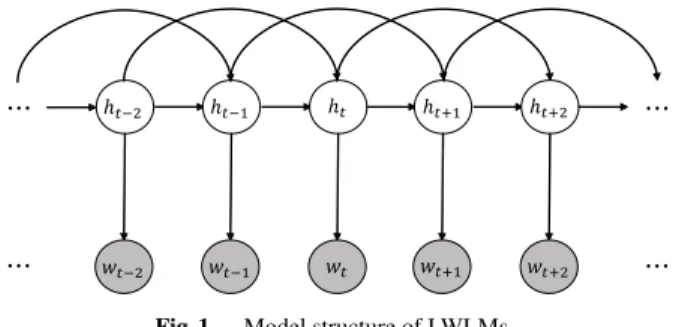
Fig. 1 Model structure of LWLMs.

2. Latent Words Language Models

2.1 Definition

LWLMs are generative models that set a latent variable for every observed word. A graphic rendering of LWLM is shown in Fig. 1. The gray circles denote observed words and the white circles denote latent variables. In the generative process of LWLM, a latent variable, called latent word ht, is generated depending on the transition probability distribution given contextlt=ht−n+1, . . . ,ht−1wherenis an n- gram order. Next, observed wordwtis generated depending on the emission probability distribution given latent wordht, i.e.,

ht∼P(ht|lt,Θlw), (1)

wt∼P(wt|ht,Θlw), (2) where Θlw is a model parameter of LWLM. P(ht|lt,Θlw) is expressed as an n-gram model for latent words, and P(wt|ht,Θlw) models the dependency between the observed word and the latent word.

An important property of LWLMs is that the latent word is expressed as a specific word that can be selected from an entire vocabulary V. Thus, the number of latent words is the same as the vocabulary size|V|. This is the reason the latent variable is called as a latent word.

2.2 Bayesian LWLMs

In the Bayesian approach, LWLM produces the following generative probability for observed wordsw=w1,· · ·,wN:

P(w)=

h

P(w|h,Θlw)P(h|Θlw)P(Θlw)dΘlw,

= N

t=1

h_t∈V

P(wt|ht,Θlw)P(ht|lt,Θlw)P(Θlw)dΘlw, (3) where h = h₁,· · ·,hN is a latent word assignment. The Bayesian approach takes account of all possible model parameters. As the integral with respect toΘlwis analytically intractable, a sampling technique is used as a feasible approximation. Eq. (3) is approximated as:

(3)

P(w) 1 M

M

m=1

P(w|Θ^m_lw)

= 1 M

M

m=1

N

t=1

ht∈V

P(wt|ht,Θ^m_lw)P(ht|lt,Θ^m_lw), (4) where Θ^m_lw means m-th point estimated model parameter.

The generative probability can be approximated usingMin- stances ofΘ^m_lw. Although we can only use one instance for the approximation, we conduct ensemble modeling (M >

1). In fact, the ensemble of several models is eﬀective for LMs such as random class-based LMs[25]and random forest LMs[8].

LWLM has a similar structure to the standard class- based n-gram model. The latent word corresponds, ap- proximately, to the class of the standard class-based n-gram model[6]. LWLM has a soft word clustering structure that diﬀers from a simple hard word clustering structure in the standard class-based n-gram model. In the hard word clustering structure, one word belongs to only one class. In the soft word clustering structure, on the other hand, one word belongs to multiple classes. Strictly speaking, each word belongs to all classes in LWLM. In addition, LWLM has vast class space about as large as the vocabulary while the number of class in the standard class-based n-gram model is often defined as several hundreds or thousands.

2.3 Training

LWLM is trained using word sequencew=w1,· · ·,wN. In LWLM training, we have to infer the latent word assignment h = h1,· · ·,hN behindw. In fact, we infer latent word as- signmentsh₁,· · ·,hM. Once a latent word assignmenthmis defined,P(wt|ht,Θ^m_lw) andP(ht|lt,Θ^m_lw) can be calculated.

To estimate the latent word assignments, Gibbs sampling is suitable. Gibbs sampling samples a new value for the latent word in accordance with its distribution and places it at positionkinh. The conditional probability distribution of possible values for latent wordhtis given by:

P(ht|w,h₋t)∝P(wt|ht,Θlw,−t)

t+n−1

j=t

P(hj|lj,Θlw,−t), (5) where h₋t represents all latent words except forht. In the sampling procedure,P(ht|lt,Θlw,−t) andP(wt|ht,Θlw,−t) can be calculated fromwandh₋t.

The transition probability distribution and the emission probability distribution are calculated on the basis of their prior distributions. For the transition probability distribution, this paper uses a hierarchical Pitman-Yor prior.

P(ht|lt,Θlw) is given as:

P(ht|lt,Θlw)=P(ht|lt,h), (6)

P(ht|lt,h)= c(ht,lt)−d_|l_t|s(ht,lt) θ|l_t|+c(lt)

+θ_|l_t|+d_|l_t|s(lt)

θ_|l_t|+c(lt) P(ht|π(lt),h), (7)

Algorithm 1: Random sampling based on trained LWLM.

Input: Model parametersΘ¹lw,· · ·,Θlw^M, number of sampled wordsN Output: Sampled wordsw

1: l1=<s>

2: fort=1 toNdo 3: m∼P(m)=M¹

4: ht∼P(ht|lt,Θ^mlw) 5: wt∼P(wt|ht,Θ^m_lw) 6: end for

7: returnw=w1,· · ·,wN

where π(lt) is the shortened context obtained by removing the earliest word fromlt.c(ht,lt) andc(lt) are counts calculated from a latent word assignmenth. s(ht,lt) ands(lt) are calculated from a seating arrangement defined by the Chi- nese restaurant franchise representation of the Pitman-Yor process[26]. d_|lt|andθ|lt|are discount and strength parameters of the Pitman-Yor process, respectively. Moreover, we use a Dirichlet prior for the emission probability distribution[27].P(wt|ht,Θlw) is given as:

P(wt|ht,Θlw)=P(wt|ht,w,h), (8)

P(wt|ht,w,h)= c(wt,ht)+αP(wt)

c(ht)+α , (9) whereP(wt) is the maximum likelihood estimation value of unigram probability in the training dataw.c(wt,ht) andc(ht) are counts calculated fromwand latent word assignmenth.

A hyper parameterαcan be optimized via a validation set.

3. N-gram Approximation of LWLMs

3.1 Sampling Based Approximation

Our idea is to convert trained LWLMs into the back-oﬀ n-gram structure. The n-gram approximation of a trained LWLM is based on random sampling of observed words. As LWLM is a generative model, it can generate latent words and observed words. Therefore, we can easily sample a lot of observed words and construct a back-oﬀn-gram model from them. The random sampling is based on Algorithm 1.

In line 1,l1is initialized as sentence head symbol<s>.

Through iterations of lines 2-6, we can obtain a large number of word sequences. WithN iterations, we can generate N latent words, and N observed words. The N observed words are used only for back-oﬀn-gram model estimation.

We define the probability distribution of the approximated model asP(wt|ut,Θlwng) where ut means context informa- tionwt−n+1, . . . ,wt−1,nis n-gram order, andΘlwngrepresents the model parameter. In fact, any back-oﬀn-gram structure, including HPYLMs, can be used for the approximation.

3.2 Linear Interpolation

It can be considered that the approximated model has properties that diﬀer from the equivalent n-gram model directly

(4)

constructed from training data because the sampled data de- rived from the trained LWLM includes various linguistic phenomena that are not present in the original training data.

Therefore, we can expect that interpolating both LMs will eﬀectively improve ASR performance. The probability distribution of interpolated n-gram modelP(wt|ut,Θmix) is defined as:

P(wt|ut,Θmix)=λP(wt|ut,Θng)

+(1−λ)P(wt|ut,Θlwng), (10) whereP(wt|ut,Θng) means the probability distribution of the n-gram model constructed from the original training data.

Interpolation weight λ can be optimized by using a validation data set. In fact, the interpolated model can be ap- proximately represented as a single back-oﬀn-gram structure[28]. The calculation can be conducted by adding both smoothed n-gram probabilities with mixture weights and re- computing back-oﬀprobabilities.

3.3 Entropy Pruning for Reducing Model Size

Our approach has a weakness in that the approximated model size becomes excessive as many words are sampled to realize an adequate approximation. To reduce model size, the entropy pruning technique can be used[29]. The entropy pruning can eﬃciently reduce the n-gram entries in the back-oﬀn-gram structure. The decision as to whether the n- gram entry (ut,wt) should be retained or pruned is based on the relative entropy between non-pruned modelP(wt|ut,Θ) and pruned model (wt|ut,Θ). Relative entropyD(Θ||Θ) is calculated by:

D(Θ||Θ)=P(ut)

wt

P(wt|ut,Θ) logP(wt|ut,Θ) P(wt|ut,Θ), (11) where P(ut) is computed using the chain rule and lower order n-gram model. A threshold for the relative entropy should be defined in accordance with the actual use case.

4. Experiment 1: Perplexity Evaluation

4.1 Setups

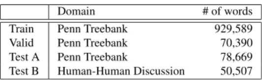
First, we conducted experiments using the Penn Treebank corpus, one of the most widely used sources for evaluating LMs[30]. Sections 0-20 were used as a training set (Train), sections 21 and 22 were used as a validation set (Valid), and Sect. s 23 and 24 were used as a test set (Test A). This se- lection matches those of many previous works. In addition, we prepared human-human discussion text data (Test B) for evaluations in a domain diﬀerent from the training set. Each vocabulary was limited to 10K words and there were no out- of-vocabulary words. Table 1 shows details.

In this evaluation, we constructed the following LMs.

• MKN5: Word-based 5-gram LM with interpolated Kneser-Ney smoothing constructed from training

Table 1 Data sets in Experiment 1.

Domain # of words

Train Penn Treebank 929,589

Valid Penn Treebank 70,390

Test A Penn Treebank 78,669

Test B Human-Human Discussion 50,507

set[3].

• HPY5: Word-based 5-gram HPYLM constructed from the training set[5]. For the training, we used 200 iterations for burn-in, and collected 10 sets of samples.

• C-HPY5: Hard class-based 5-gram HPYLM constructed from training set. Brown clustering was used for deciding word class[6]. The class size was 1K.

• RNN: Word-based RNNLM[10]. The hidden layer size was set as 200 by referring to a preliminary experiment.

• A-HPY5: Word-based 5-gram HPYLM constructed from data generated on the basis ofHPY5.

• RNN5: Word-based 5-gram HPYLM constructed from data generated on the basis ofRNN[21].

• LW5: Word-based 5-gram HPYLM constructed from data generated on the basis of 5-gram LWLM constructed from training set. For training LWLM, we used 500 iterations for burn-in, and collected 10 samples.

In addition, we employed several mixed models constructed by linearly interpolating the above LMs. For example, HPY5+LW5 is a mixed model constructed from HPY5 and LW5. The mixture weights were optimized using a validation set on the basis of the EM algorithm. Other hyper parameters were also optimized using the validation set.

4.2 Results

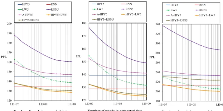
For the n-gram approximation approaches (A-HPY5,RNN5, LW5), the generated data size is related to the performance of the approximated models. Therefore, we investigated the relationship between the data size generated by random sampling and perplexity (PPL) reduction in the validation set and each test set. We constructed each approximated model, and mixed models (RNN5+HPY5,LW5+HPY5) by varying the generated data size and computed the corresponding PPL.

We plot the results along with the results ofHPY5andRNN in Fig. 2, where the horizontal axis is in log-scale.

Figure 2 shows that the PPL of each model was reduced as the generated data increased. InA-HPY5, PPL con- verged with just a small amount of generated data because HPYLM has a simple model structure.A-HPY5matched the performance of HPY5 in each data set when a lot of data was generated. On the other hand, inRNN5andLW5, more generated data was necessary for PPL convergence than in A-HPY5. LW5outperformed A-HPY5andRNN5 when a lot of data was generated. RNN5 could not match the performance of the originalRNN. This is because the back-oﬀn- gram structure cannot take into account long-range context although RNNLM can consider the long-range context dis-

(5)

Fig. 2 Relations between data size generated by random sampling and perplexity in Experiment 1.

Table 2 Perplexity results in Experiment 1.

Valid Test A Test B

1. MKN5 148.0 141.2 238.6

2. HPY5 145.1 139.3 232.7

3. C-HPY5 150.8 142.2 237.0

4. A-HPY5 147.1 141.1 233.3

5. RNN5 160.4 150.4 286.4

6. LW5 138.7 131.7 205.5

7. HPY5+RNN5 130.5 124.5 226.7 8. HPY5+LW5 128.6 123.1 200.8

9. RNN 134.4 128.9 212.9

10. HPY5+RNN 111.4 107.9 180.6 11. HPY5+RNN5+RNN 113.4 109.2 186.8 12. HPY5+LW5+RNN 109.8 105.4 175.8

tributed representation of words.

In addition, both mixed models also experienced im- provements in PPL performance as the generated data size increased. Although the isolated use ofRNN5was not effective, its combination withHPY5yielded improved PPL performance. Also, LW5performance was improved through combination withHPY5. This combination was effective because the data generated on the basis of RNNor LW have different attributes from the original training data. The combination ofHPY5andA-HPY5did not improve performance because they were almost the same (the results are not shown in Fig. 2).

Next, we investigated PPL performance for all LMs;

the generated data size was set to 1 giga (1.E+09) words for A-HPY5,RNN5andLW5. The results are shown in Table 2.

Lines 1-6 show the results for the back-oﬀ n-gram structure. In each data set,LW5achieved the best results.

Note thatC-HPY5could not achieve better results thanLW5.

Thus, the simple hard clustering structure does not im-

prove PPL performance for either in-domain data or out-of- domain data, and LWLM structure (soft clustering with vast class size) seems to be eﬀective for domain robustness.

Lines 7 and 8 show the results for the mixed n-gram models that can also be expressed as simple back-oﬀn-gram structures. The combination ofHPY5andRNN5orLW5could improve PPL performance more than their isolated use. In each data set,HPY5+LW5was superior toHPY5+RNN5. It can be considered that the performance was improved because LW5had diﬀerent attributes fromHPY5.

Lines 9-12 show the results forRNNand its combination with the back-offn-gram structure.RNNoutperformed other isolated models (lines 1-6) for the validation set and test set A. On the other hand,LW5was superior toRNNfor test set B althoughLW5has a back-offn-gram structure. The combi- nations ofRNNwith the models with back-offn-gram structure were effective. In each data set, the best results were obtained byHPY5+LW5+RNN. This shows that performance can be improved by n-gram approximation of LWLM even if RNNLM is also used.

Additionally, we investigated the properties of each approximated model to reveal thatLW5was more eﬀective than A-HPY5 and RNN5. Table 3 shows the number of 3- and 5-gram entries in each model and n-gram hit rate for the validation set and each test set. The hit rate represents the percentage of n-gram entries in the reference data that are explicitly listed in the LMs. We calculated 3-gram hit rate (N≥3), which includes the high order (4-gram and 5-gram) hit rate and 5-gram hit rate (N=5); the generated data sizes of each model were set to 10M, 100M and 1000M.

Table 3 shows thatLW5had a lot more n-gram entries than A-HPY5 and RNN5 for the same generated data size.

This means that random sampling based on LWLM can gen-

(6)

Table 3 Number of n-gram entries and n-gram hit rate [%] results in Experiment 1.

Data size # of 3-gram # of 5-gram Valid Test A Test B

N≥3 N=5 N≥3 N=5 N≥3 N=5

HPY5 930K 586558 737952 39.58 8.62 40.26 7.43 29.01 0.81

A-HPY5 10M 5663883 8848534 49.33 9.80 50.51 8.77 44.62 1.84 100M 40649386 83207920 62.53 14.40 64.28 13.71 61.06 4.91 1000M 274813830 760971607 74.83 19.83 76.61 20.68 75.61 10.54

RNN5 10M 4905245 7768561 47.75 8.75 48.86 7.92 37.49 1.07

100M 33458232 72434311 62.30 13.54 64.02 12.92 55.24 3.18 1000M 219833882 665415678 74.77 19.98 76.75 19.83 71.62 7.62

LW5 10M 6608797 9409511 50.40 9.33 51.62 8.27 46.22 1.69

100M 48464818 90136805 65.28 14.16 67.45 13.58 64.77 4.74 1000M 319956811 841974035 77.45 20.98 79.41 21.14 78.84 10.82

erate a greater variety of linguistic phenomena than HPYLM or RNNLM. In addition, the 3-gram hit rate and 5-gram hit rate ofLW5were superior to those ofA-HPY5andRNN5for each data set. This means that random sampling based on LWLM can generate words that are actually in the data set.

These results show that an approximated model based on eﬀective random sampling can perform robustly in multiple domains.

5. Experiment 2: ASR Evaluation

5.1 Setups

The second experiments used the Corpus of Spontaneous Japanese (CSJ) for ASR evaluation[31]. We divided CSJ into a training set (Train), a small validation set (Valid), and a test set (Test A). Vocabulary size of the training set was 83,536. The validation set was used in optimizing the hyper parameters of the LMs. In addition, a contact center dialog task (Test B) and a voice mail task (Test C) were prepared for evaluation in out-of-domain environments. In the contact center dialogue task, two speakers, an operator and a customer, talked to each other as in call center dialogs.

Twenty four phone calls (24 operator channels and 24 customer channels) were used in the evaluation. In the voice mail task, a person left small voice messages using a smart phone, and 237 messages were used in the evaluation. Ta- ble 4 shows details.

For speech recognition evaluation, we prepared an acoustic model on the basis of hidden Markov models with deep neural networks (DNN-HMM)[32]. The DNN-HMM had eight hidden layers with 2048 nodes and was trained using the CSJ training set. The speech recognition decoder was VoiceRex, a WFST-based decoder[33], [34]. JTAG was used as the morpheme analyzer to split sentences into words[35].

In this evaluation, we constructed the following LMs.

• MKN3: Word-based 3-gram LM with interpolated Kneser-Ney smoothing constructed from training set[3].

• HPY3: Word-based 3-gram HPYLM constructed from the training set[5]. For the training, we used 200 iterations for burn-in, and collected 10 samples.

Table 4 Data sets in Experiment 2.

Domain # of words

Train Lecture 7,317,392

Valid Lecture 28,046

Test A Lecture 27,907

Test B Contact center 24,665 Test C Voice mail 21,044

• C-HPY3: Hard class-based 3-gram HPYLM constructed from training set. Brown clustering was used for deciding word class. The class size was 5K[6].

• RNN: Class-based RNNLM with 500 hidden nodes and 500 classes[11].

• A-HPY3: Word-based 3-gram HPYLM constructed from 1000M data generated on the basis ofHPY3.

• RNN3: Word-based 3-gram HPYLM constructed from 1000M data generated on the basis ofRNN.

• LW3: Word-based 3-gram HPYLM constructed from data generated on the basis of 3-gram LWLM constructed from training set. For the training of LWLM, we used 500 iterations for burn-in and collected 10 samples.

In addition, we examined several mixed models constructed from the above LMs by linear interpolation. The mixture weights were optimized using the validation set and the EM algorithm. Other hyper parameters were also optimized using the validation set. These LMs, except forRNN, can be represented using ARPA format, a standard back-oﬀn-gram format, and they can be directly introduced to WFST decoders. RNNcan be used as a rescoring model that is introduced after decoding. For rescoring, we generated 1000- best lists in the decoding pass. For example,HPY3+LW3was used for decoding to generate the recognition hypotheses when we examinedHPY3+LW3+RNN.

5.2 Results

Table 5 shows the PPL and word error rate (WER) results for each condition. PPL was only evaluated in RNNsince RNNLMs cannot be applied to ASR directly.

Lines 1-6 show the results for the back-oﬀ n-gram structure. HPY3 outperformed MKN3 andC-HPY3 in terms of PPL and WER. AlthoughC-HPY3yielded dimensionality

(7)

Table 5 Perplexity and word error rate [%] results in Experiment 2.

Valid Test A Test B Test C

(In-Domain) (In-Domain) (Out-Of-Domain) (Out-Of-Domain)

PPL WER PPL WER PPL WER PPL WER

1. MKN3 81.38 19.98 69.36 24.79 167.61 38.67 189.93 32.00

2. HPY3 79.32 19.74 67.50 24.67 158.13 38.29 175.63 31.69

3. C-HPY3 82.97 19.91 69.36 24.59 158.92 38.39 180.89 32.17 4. A-HPY3 82.69 20.20 70.43 25.23 161.56 38.82 177.61 32.04

5. RNN3 98.65 21.63 82.23 26.24 153.89 39.32 163.99 31.96

6. LW3 79.57 19.61 66.93 24.54 141.34 36.93 147.87 30.42

7. HPY3+RNN3 77.96 19.53 66.09 24.26 143.88 37.60 149.81 30.18 8. HPY3+LW3 72.86 18.65 62.05 23.58 134.65 35.99 141.23 28.74

9. RNN 69.49 - 60.78 - 145.05 - 158.57 -

10. HPY3+RNN 64.01 18.53 55.84 23.45 122.52 37.45 142.62 30.89 11. HPY3+RNN3+RNN 63.76 18.41 55.77 23.12 119.00 36.85 138.54 29.24 12. HPY3+LW3+RNN 61.56 17.85 53.36 22.68 114.71 35.36 133.09 28.06

Table 6 Perplexity and word error rate [%] results of pruned models in Experiment 2.

Size Valid Test A Test B Test C

(In-Domain) (In-Domain) (Out-Of-Domain) (Out-Of-Domain)

PPL WER PPL WER PPL WER PPL WER

HPY3 322 M 79.32 19.74 67.50 24.67 158.13 38.29 175.63 31.69

HPY3+LW3 22.0 G 72.86 18.65 62.05 23.58 134.65 35.99 141.23 28.74 9.8 G 73.39 18.70 62.86 23.56 135.02 36.01 143.05 28.63 3.9 G 73.74 18.53 63.21 23.60 135.47 36.05 143.91 28.76 2.2 G 74.09 18.58 63.51 23.67 136.02 36.13 144.44 28.81 563 M 75.41 18.75 64.69 23.87 137.86 36.50 147.66 28.91 353 M 76.39 18.81 65.46 23.78 138.95 36.49 149.08 28.78

reduction and smoothing,C-HPY3performed comparably or inferiorly toHPY3. Among approximated models,LW3per- formed the best in terms of PPL and WER. For the validation set and test set A,LW3was comparable toHPY3. On the other hand, for test sets B and C,LW3performed remarkably better than HPY3. This result shows that LWLM robustly handles speech domains diﬀerent from that of the training data. It seems that the learning criteria, which identify related words, are eﬀective in expanding the application range of LMs. These results correspond to those in Experiment 1.

Lines 7 and 8 show the results of mixed n-gram models that can be also used for WFST-based one-pass decoding.

HPY3+LW3was superior toHPY3+RNN3in all data sets. We obtained better WER reduction fromHPY3+LW3thanHPY3 orLW3. Although the mixture weight ofHPY3+LW3was optimized for the validation data, the mixed model performed robustly in out-of-domain data sets.

Lines 9-12 show the results of RNN and the combination with back-off n-gram structure. RNN was superior toHPY3 and LW3in the validation set and test set A. On the other hand, in test sets B and C,RNN was inferior to LW3. LW3 seems to be robust at supporting multiple domains. Lines 10-12 compare rescored results usingRNNaf- ter WFST-based decoding with back-offn-gram structure in terms of ASR performance. For example, in line 12, decoding was based on HPY3+LW3and 1000-best rescoring was based onHPY3+LW3+RNN. Combining RNN with the back- off n-gram structure improved PPL and WER. The highest result was obtained byHPY3+LW3+RNNin all data sets.

These results suggest that WFST-based decoding perfor-

mance must be improved for utilizing an intelligent rescoring model such as RNNLM.

Next, we applied entropy pruning to HPY3+LW3, the combination with the highest performance among the back- oﬀ n-gram structures[29]. We investigated the relationship between model size and the performance of the pruned model variants. Model size is taken to be ARPA file size with ASCII format.

The results in Table 6 show that entropy pruning could reduce model size eﬃciently. Even if we reduced the model size of HPY3+LW3 such that it was comparable to that of HPY3,HPY3+LW3was superior toHPY3in terms of PPL and WER. Especially, in out-of-domain data, the pruned models outperformedHPY3. These results show that entropy pruning is suitable for introducing our approach to practical ASR systems.

6. Conclusions

In this paper, we proposed an n-gram approximation of LWLM for improving ASR performance in multiple domains. Our approach allows LWLM to support one-pass ASR decoding by converting it into the back-off n-gram structure. We revealed that random sampling based on LWLM can generate various linguistic phenomena and that the back-offn-gram model constructed from the generated data performs robustly in not only in-domain data but also out-of-domain data. We also showed that the interpolation of approximated model and standard n-gram model effectively improves ASR performance. Moreover, we revealed

(8)

that entropy pruning is useful in reducing constructed model size even though a lot of data is needed to adequately approximate LWLM.

References

[1] J.T. Goodman, “A bit of progress in language modeling,” Computer Speech & Language, vol.15, pp.403–434, 2001.

[2] S.F. Chen and J. Goodman, “An empirical study of smoothing techniques for language modeling,” Computer Speech & Language, vol.13, pp.359–383, 1999.

[3] R. Kneser and H. Ney, “Improved backing-oﬀfor m-gram language modeling,” Proc. ICASSP, vol.1, pp.181–184, 1995.

[4] Y.W. Teh, “A hierarchical Bayesian language model based on Pitman-Yor processes,” Proc. COLING/ACL, pp.985–992, 2006.

[5] S. Huang and M. Yor, “Hierarchical Pitman-Yor language models for ASR in meetings,” Proc. ASRU, pp.124–129, 2007.

[6] P.F. Brown, P.V. deSouza, R.L. Mercer, V.J.D. Pietra, and J.C. Lai,

“Class-based n-gram models of natural language,” Computational Linguistics, vol.18, pp.467–479, 1992.

[7] G. Potamianos and F. Jelinek, “A study of n-gram and decision tree letter language modeling methods,” Speech Communication, vol.24, no.3, pp.171–192, 1998.

[8] P. Xu and F. Jelinek, “Random forests in language modeling,” Proc.

EMNLP, pp.325–332, 2004.

[9] Y. Bengio, R. Ducharme, P. Vincent, and C. Jauvin, “A neural prob- abilistic language model,” J. Mach. Learn. Res., vol.3, pp.1137–

1155, 2003.

[10] T. Mikolov, M. Karafiat, L. Burget, J. Cernocky, and S. Khudanpur,

“Recurrent neural network based language model,” Proc. INTER- SPEECH, pp.1045–1048, 2010.

[11] T. Mikolov, S. Kombrink, L. Burget, J. Cernocky, and S. Khudanpur,

“Extensions of recurrent neural network language model,” Proc.

ICASSP, pp.5528–5531, 2011.

[12] K. Deschacht, J.D. Belder, and M.-F. Moens, “The latent words language model,” Computer Speech & Language, vol.26, pp.384–409, 2012.

[13] S. Goldwater and T. Griﬃths, “A fully Bayesian approach to unsupervised part-of-speech tagging,” Proc. ACL, pp.744–751, 2007.

[14] P. Blunsom and T. Cohn, “A hierarchical Pitman-Yor process HMM for unsupervised part of speech induction,” Proc. ACL, pp.865–874, 2011.

[15] Y. Su, “Bayesian class-based language models,” Proc. ICASSP, pp.5564–5567, 2011.

[16] J.-T. Chien and C.H. Chueh, “Dirichlet class language models for speech recognition,” IEEE Transactions on Audio, Speech and Lan- guage Processing, vol.19, pp.482–495, 2011.

[17] W. Wang, A. Stolcke, and M.P. Harper, “The use of a linguisti- cally motivated language model in conversational speech recognition,” Proc. ICASSP, pp.261–264, 2004.

[18] R. Wang, M. Utiyama, I. Goto, E. Sumita, H. Zhao, and B.L. Lu,

“Converting continuous-space language models into n-gram language models for statistical machine translation,” Proc. EMNLP, pp.845–850, 2013.

[19] E. Arisoy, S.F. Chen, B. Ramabhadran, and A. Sethy, “Converting neural network language models into back-oﬀlanguage models for eﬃcient decoding in automatic speech recognition,” Proc. ICASSP, pp.8242–8246, 2013.

[20] E. Arisoy, S.F. Chen, B. Ramabhadran, and A. Sethy, “Convert- ing neural network language models into back-oﬀlanguage models for eﬃcient decoding in automatic speech recognition,” IEEE/ACM Trans. Audio, Speech, Language Process., vol.22, pp.2329–9290, 2014.

[21] A. Deoras, T. Mikolov, S. Kombrink, M. Karafiat, and S.

Khudanpur, “Variational approximation of long-span language models in LVCSR,” Proc. ICASSP, pp.5532–5535, 2011.

[22] A. Deoras, T. Mikolov, S. Kombrink, and K. Church, “Approximate inference: A sampling based modeling technique to capture complex dependencies in a language model,” Speech Communication, vol.55, no.1, pp.162–177, 2013.

[23] H. Adel, K. Kirchhoff, N.T. Vu, D. Telaar, and T. Schultz, “Com- paring approaches to convert recurrent neural networks into back- offlanguage models for efficient decoding,” Proc. INTERSPEECH, pp.651–655, 2014.

[24] R. Masumura, H. Masataki, T. Oba, O. Yoshioka, and S. Takahashi,

“Use of latent words language models in ASR: a sampling-based implementation,” Proc. ICASSP, pp.8445–8449, 2013.

[25] A. Emami and F. Jelinek, “Random clusterings for language modeling,” Proc. ICASSP, vol.1, pp.581–584, 2005.

[26] Y.W. Teh, M.I. Jordan, M.J. Beal, and D.M. Blei, “Hierarchical Dirichlet processes,” Journal of the American Statistical Associa- tion, vol.101, no.476, pp.1566–1581, 2006.

[27] D.J.C. MacKay and L.C. Peto, “A hierarchical Dirichlet language model,” Natural Language Engineering, vol.1, pp.289–308, 1994.

[28] A. Stolcke, “SRILM – an extensible language modeling toolkit,”

Proc. ICSLP, vol.2, pp.901–904, 2002.

[29] A. Stolcke, “Entropy-based pruning of backoﬀlanguage models,”

Proc. DARPA Broadcast News Transcription and Understanding Workshop, pp.270–274, 1998.

[30] M.P. Marcus, M.A. Marcinkiewicz, and B. Santorini, “Building a large annotated corpus of English: The penn treebank,” Computa- tional Linguistics, vol.19, pp.313–330, 1993.

[31] K. Maekawa, H. Koiso, S. Furui, and H. Isahara, “Spontaneous speech corpus of Japanese,” Proc. LREC, pp.947–952, 2000.

[32] G. Hinton, L. Deng, D. Yu, G. Dahl, A.-R. Mohamed, N. Jaitly, A. Senior, V. Vanhoucke, P. Nguyen, T. Sainath, and B. Kingsbury,

“Deep neural networks for acoustic modeling in speech recognition,” IEEE Signal Process. Mag., vol.29, no.6, pp.82–97, 2012.

[33] T. Hori, C. Hori, Y. Minami, and A. Nakamura, “Eﬃcient WFST- based one-pass decoding with on-the-fly hypothesis rescoring in extremely large vocabulary continuous speech recognition,” IEEE transactions on Audio, Speech and Language Processing, vol.15, no.4, pp.1352–1365, 2007.

[34] H. Masataki, D. Shibata, Y. Nakazawa, S. Kobashikawa, A. Ogawa, and K. Ohtsuki, “VoiceRex spontaneous speech recognition technology for contact-center conversations,” NTT Technical Review, vol.5, no.1, pp.22–27, 2007.

[35] T. Fuchi and S. Takagi, “Japanese morphological analyzer using word co-occurrence: JTAG,” Proc. COLING/ACL, pp.409–413, 1998.

(9)

Ryo Masumura received B.E. and M.E.

degrees in engineering from Tohoku University, Sendai, Japan, in 2009 and 2011, respectively.

Since joining Nippon Telegraph and Telephone Corporation (NTT) in 2011, he has been engaged in research on speech recognition, spoken language processing, and natural language processing. He received the Student Award and the Awaya Kiyoshi Science Promotion Award from the Acoustic Society of Japan (ASJ) in 2011 and 2013, respectively, the Sendai Section Student Awards The Best Paper Prize from the Institute of Electrical and Electron- ics Engineers (IEEE) in 2011, the Yamashita SIG Research Award from the Information Processing Society of Japan (IPSJ) in 2014, the Young Researcher Award from the Association for Natural Language Processing (NLP) in 2015, and the ISS Young Researcher’s Award in Speech Field from the Institute of Electronic, Information and Communication Engi- neers (IEICE) in 2015. He is a member of the ASJ, the IEICE, the IPSJ, the NLP, the IEEE, and the International Speech Communication Association (ISCA).

Taichi Asami received B.E. and M.E. degrees in computer science from Tokyo Institute of Technology, Tokyo, Japan, in 2004 and 2006, respectively. Since joining Nippon Telegraph and Telephone Corporation (NTT) in 2006, he has been engaged in research on speech recognition and spoken language processing. He received the Awaya Kiyoshi Science Promotion Award and the Sato Prize Paper Award from the Acoustic Society of Japan (ASJ) in 2012 and 2014, respectively. He is a member of the ASJ, the Institute of Electronics, Information and Communication Engineers (IEICE), Institute of Electrical and Electronics Engineers (IEEE), and the International Speech Communication Association (ISCA).

Takanobu Oba received B.E. and M.E. degrees from Tohoku University, Sendai, Japan, in 2002 and 2004, respectively. In 2004, he joined Nippon Telegraph and Telephone Cor- poration (NTT), where he was engaged in the research and development of spoken language processing technologies including speech recognition at the NTT Communication Science Lab- oratories, Kyoto, Japan. In 2012, he started the research and development of spoken appli- cations at the NTT Media Intelligence Labora- tories, Yokosuka, Japan. Since 2015, he has been engaged in development of spoken dialogue services at the NTT Docomo Corporation, Yokosuka, Japan. He received the Awaya Kiyoshi Science Promotion Award from the Acoustical Society of Japan (ASJ) in 2007. He received Ph. D.(Eng.) degree from Tohoku University in 2011. He is a member of the Institute of Electrical and Electronics Engineers (IEEE), the Institute of Electronics, Information, and Communication Engineers (IEICE) and the ASJ.

Hirokazu Masataki received B.E., M.E., and Ph.D. degrees from Kyoto University in 1989, 1991, and 1999, respectively. From 1995 to 1998, he worked with ATR Inter- preted Telecommunications Research Labora- tories, where specialized in statistical language modeling for large vocabulary continuous speech recognition. He joined Nippon Telegraph and Telephone Corporation (NTT) in 2004 and has been engaged in the practical use of speech recognition. He received the Maejima Hisoka Award from the Tsushin-bunko Association in 2013, and the 54-th Sato Prize Paper Award from the Acoustic Society of Japan (ASJ) in 2014.

He is a member of the Institute of Electronics, Information and Communi- cation Engineers (IEICE) and the ASJ.

Sumitaka Sakauchi received M.S. degree from Tohoku University in 1995 and Ph.D. degree from Tsukuba University in 2005. Since joining Nippon Telegraph and Telephone Cor- poration (NTT) in 1995, he has been engaged in research on acoustics, speech and signal processing. He is now Senior Manager in the Re- search and Development Planning Department of NTT. He received the Paper Award from the Institute of Electronics, Information and Com- munication Engineers (IEICE) in 2001, and Awaya Kiyoshi Science Promotion Award from the Acoustic Society of Japan (ASJ) in 2003. He is a member of the IEICE and the ASJ.

Satoshi Takahashi received B.E., M.E., and Ph.D. degrees in information science from Waseda University, Tokyo, in 1987, 1989, and 2002, respectively. Since joining Nippon Tele- graph and Telephone (NTT) Corporation in 1989, he has been engaged in speech recognition, spoken dialog system, and pattern recognition. He received the Awaya Kiyoshi Sci- ence Promotion Award and the Sato Prize Pa- per Award from the Acoustic Society of Japan (ASJ) in 1992 and 2014, respectively, and the Takayanagi Kenjiro Achievement Prize form the Takayanagi Memorial Foundation for Electronics Science and Technology in 2014. He is now Vice President in NTT Media Intelligence Laboratories. He is a member of the Acoustic Society of Japan (ASJ), the Institute of Electronics, Informa- tion and Communication Engineers (IEICE), the Information Processing Society of Japan (IPSJ) and Institute of Electrical and Electronics Engi- neers (IEEE).