1330 IEICE TRANS. FUNDAMENTALS, VOL.E102–A, NO.9 SEPTEMBER 2019
LETTER
Geometric Dilution of Precision for Received Signal Strength in the Wireless Sensor Networks
Wanchun LI†a), Yifan WEI†, Ping WEI†, Hengming TAI††, Xiaoyan PENG†,Nonmembers, andHongshu LIAO†,Member
SUMMARY Geometric dilution of precision (GDOP) is a measure showing the positioning accuracy at different spatial locations in location systems. Although expressions of GDOP for the time of arrival (TOA), time difference of arrival (TDOA), and angle of arrival (AOA) systems have been developed, no closed form expression of GDOP are available for the received signal strength (RSS) system. This letter derives an explicit GDOP expression utilizing the RSS measurement in the wireless sensor networks.
key words: geometric dilution of precision, received signal strength systems
1. Introduction
GDOP is an indicator that provides the information regard- ing the degree of location accuracy affected by the geometric relation between the source(s) and the sensors[1]. The re- ceived signal strength (RSS) measurements are important and commonly used in indoor location solutions based on Wi-Fi, cellular net-works or Bluetooth[2]–[4],[8]. There- fore, it is significant to do quantitative analysis of GDOP in the RSS positioning systems. When RSS are used to estimate the source locations, the positioning accuracy is related to the accuracy of RSS measurement as well as the geometric relation between the source and the sensors[8].
This letter investigates the effect of geometric relation to the positioning accuracy based on RSS positioning systems in 3 different scenarios. In particular, the root mean square (RMS) position error is used as GDOP in the RSS system.
RSS is commonly expressed in terms of the unknown emitting source power, the priori path loss parameter (PLP) and the distance between the sensors and source. The first two parameters are independent of the geometric relation between the source and the sensors. GDOP in GPS system was calculated by considering all the errors generated by different parameters of TOA measurements[5]. In actual project the parameters are difficult to obtain normally and the GDOP with unknown parameters is different from the GDOP with known parameters. Therefore, three expressions of GDOP are derived in this letter. One is for the condition that PLP and the source power are known. The second GDOP is under the known PLP, and the third one is for unknown
Manuscript received April 10, 2019.
Manuscript revised May 9, 2019.
†The authors are with School of Electronic Engineering, Uni- versity of Electronic Science and Technology of China, Chengdu 611731, PRC.
††The author is with The University of Tulsa, Tulsa 74101, USA.
a) E-mail: [email protected] DOI: 10.1587/transfun.E102.A.1330
PLP and unknown source power.
The innovation of this letter is as follows: this letter utilizes the calculating formula of CRB to calculate GDOP, which follows the thought in paper [7]. This letter first deduces expressions of GDOP based on RSS systems in 3 different scenarios and closed form expressions for the first and second scenarios.
2. Derivation of GDOP
The signal strength received by the sensorkcan be defined as[6]
Pk =η0−10αlog10dk +nkβ (1) fork=1,2· · ·,K. P0is the unknown emitting source power andη0=P0+10αlog10d0is the equivalent unknown emit- ting source power. dk =|u−xk|is the distance between the kthsensor and the source.αis PLP andnkβis independently identically distributed (i.i.d.) Gaussian noise with zero mean and varianceσ2β.
GDOP can be obtained by connecting the contour lines of CRB on the area of interest according to the relationship between CRB and GDOP [7]. The CRB for RSS-based localization provided in [8] is an approximate expression, not in the closed form. Thus, the provided CRBs are not exact values.
The signal strength of Eq. (1) can be rewritten as nkβ=c(lnPk−αlndk−lnη0) (2) The set of all the measurements is denoted as β = cf
lnP1 . . . lnPKgT
andc=10/ln 10. The conditional probability of the measurement error can be expressed as[8]
p(ζ|u, η0, α) = const·exp
1 2σ2β
β−hβ(u, η0, α)T
β−hβ(u, η0, α)
(3) where const is a constant independent of the localization parameters(u, η0, α). In Eq. (3),hβcan be expressed as
hβ(u, η0, α)=c
αlnd1+lnη0 ... αlndk+lnη0
(4)
Copyright © 2019 The Institute of Electronics, Information and Communication Engineers
LETTER
1331
The Fisher matrix can be constructed by[7],[8]
FIM=H Q−1H (5)
where H=f
Hβu Hηβ0 HαβgT
(6)
Q=σβ2I (7)
Hβu =∂hTβ
∂u =cα
"
d−11cosθ1 · · · d−K1 cosθK d1−1sinθ1 · · · d−K1 sinθK
# (8)
Hηβ0= ∂hTβ
∂η0 =cη−01f
1 · · · 1g
=cη−01·1T (9)
Hβα =∂hTβ
∂α =cf
lnd1 · · · lndKg
. (10)
The CRB of location parameters with respect to power is shown as[8]
CRB=(FIM)−1. (11)
The CRB1 of the localization with knownη0 andα is ob- tained from Eq. (11) and can be expressed as
CRB1 =
HβuQ−1HβTu
−1
. (12)
The 1stGDOP is defined as[7]
GDOP1=p
tr(CRB1), (13)
where tr(X)is the trace of matrixX. After arrangement, we have
GDOP1= σβ cα
* ,
XK
k=1
d−k2+ -
/A
−1/2
(14) where
A=
K
X
k=1 K
X
m,k
sin2(θk −θm)d−k2d−m2
−1
(15) The CRB of the localization with knownαcan be derived from Eq. (11)
CRB2 =σ2β Huβ
I−(1/K)11T HβuT−1
(16) The 2ndGDOP is defined as[7]
GDOP2=p
tr(CRB2) (17)
After some manipulations, we have GDOP2 =
A
K
X
k=1
d−k2+A2·f
(B·F−C·E)2+(C·
F−B·D)2g
/[K−A·G]
1/2
·σβ/(cα) (18)
Fig. 1 GDOP for RSS with 24 sensors and positive hexagon distribution.
* denotes the sensor. a: GDOP1, b: GDOP2, c: GDOP3
B=
K
X
k=1
cosθkd−k1 (19)
C=
K
X
k=1
sinθkdk−1 (20)
D=
K
X
k=1
sin2θkd−k2 (21)
E=
K
X
k=1
cos2θkd−k2 (22)
F=
K
X
k=1
cosθksinθkd−k2 (23)
1332 IEICE TRANS. FUNDAMENTALS, VOL.E102–A, NO.9 SEPTEMBER 2019
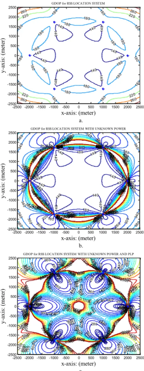
Fig. 2 GDOP for RSS with 6 sensors and positive hexagon distribution.
a: GDOP1, b: GDOP2, c: GDOP3
G= XK
m=1
[Bsinθm−Ccosθm]2d−m2. (24) Similarly, the CRB of the localization with unknownη0and αcan be derived as
CRB3=σβ2
"
Huβ HβuT
−Hβu HaβT
Haβ
HβaT−1
Hβa
Haβ
T#
(25) where
Hβa =f
Hβη0 HαβgT
(26) The 3rdGDOP is defined as
GDOP3=p
tr(CRB3) (27)
3. Simulation Study
Two scenarios of GDOP for received signal strength are ex- amined. In scenario 1, 24 sensors are set as the cellular layout (positive hexagon) with side length of 1 km and marked with
* symbols in the figure. The RSS measurement errornkβis the white Gaussian noise with zero mean and 2 dB variance.
The propagation factorαis set as 2. Scenario 2 has the same layout as scenario 1, but with only 6 sensors. The variance of RSS measurement error is 1 dB andαis 3.
Figure 1 shows the contour maps of the RSS localization for scenario 1. Figure 1a is for GDOP1, Fig. 1b for GDOP2, and Fig. 1c for GDOP3. It can be seen from Fig. 1 that the positioning accuracy is between 110 and 170 meters in most regions whether or not the equivalent source power η0and the PLP are unknown. Close examination of Fig. 1a, 1b, and 1c shows that the positioning error along the anchor-anchor line gradually increases along with the increase of unknown conditions.
Figure 2 illustrates the contour maps of the RSS lo- calization for scenario 2. It can be seen from Fig. 2a that the positioning accuracy is satisfactory when PLP and the source power are known. It is observed from Fig. 2b and Fig. 2c that the RSS localization results deteriorate rapidly along and off the anchor-anchor line, and become irregular when both PLP and source power are not known.
4. Conclusion
Three GDOP expressions for RSS-based positioning systems are presented. Simulation results for different number of sensors are given to illustrate the effects of the GDOP.
References
[1] D.J. Torrieri, “Statistical theory of passive location systems,” IEEE Trans. Aerosp. Electron. Syst., vol.AES-20, no.2, pp.183–198, March 1984.
[2] S. Fang, Y. Hsu, Y. Shiao, and F. Sung, “An enhanced device local- ization approach using mutual signal strength in cellular networks,”
IEEE Internet Things J., vol.2, no.6, pp.596–603, Dec. 2015.
[3] G. Wang and K. Yang, “A new approach to sensor node localization using RSS measurements in wireless sensor networks,” IEEE Trans.
Wireless Commun., vol.10, no.5, pp.1389–1395, May 2011.
[4] Y.I. Wu, H. Wang, and X. Zheng, “WSN localization using RSS in three-dimensional space — A geometric method with closed-form solution,” IEEE Sensors J., vol.16, no.11, pp.4397–4404, June, 2016.
[5] M.V. Desai, D. Jagiwala, and S.N. Shah, “Impact of dilution of pre- cision for position computation in Indian regional navigation satellite system,” Proc. 2016 Int’l Conf. Advances in Computing, Commun.
Informatics (ICACCI), pp.980–986, Jaipur, 2016.
[6] T.S. Rappaport, Wireless Communications: Principles and Practice, Prentice-Hall, Upper Saddle River, NJ, USA, 1996.
[7] W.C. Li, T. Yuan, and B. Wang. “GDOP and the CRB for positioning systems,” IEICE Trans. Fundamentals, vol.E100-A, no.2, pp.733–737.
Feb. 2017.
[8] M. Angjelichinoski, D. Denkovski, V. Atanasovski, and L.
Gavrilovska, “Cramér–Rao lower bounds of RSS-based localization with anchor position uncertainty,” IEEE Trans. Inf. Theory, vol.61, no.5, pp.2807–2834, May 2015.