Four Essays in Nonlinear Economic Dynamics

(1)

Four Essays in Nonlinear Economic Dynamics

A Dissertation

Presented to Graduate School of

Humanities and Social Sciences Doctor’s Course

Okayama University

In partial Fulfillment

of the Requirements for the Degree Doctor of Philosophy in Economics

by

Yosuke Umezuki

March 2019

(2)

Preface

In the mid-20th century, N. Kaldor, R. M. Goodwin, J. R. Hicks, and others studied the autonomous and sustainable economic fluctuations caused by the nonlinearity inherent in an economy. The research field that emerged can be called either the “theory of nonlinear business cycles” or the “theory of endogenous business cycles.” A major reason for the popularity of these studies was the progress made in the theory of nonlinear oscillations, which was then being actively pursued in science and engineering.

However, the nonlinear oscillation theory–or at least the kind practiced by the economists of that era–was mainly concerned with relatively simple vibration patterns, such as limit cycles in a continuous time system. Thus, such studies proved inadequate in identifying those characteristics of the economy that are recurrent but not periodic. In addition, after the “microfundations” began to be used widely for research in the latter half of the 20th century, studies of nonlinear dynamics in economics, which often lacked microfoundations, eventually got sidelined by more mainstream topics in economics.

In stark contrast to the “decline” in use of nonlinear dynamics in economics, research related to autonomous fluctuations of dynamical systems has been vigorously pursued since the 20th century in the mathematical sciences as “dynamical system theory.” The growing interest in a complex nonlinear phenomenon called chaos is a particularly signif- icant development. The term chaos became popular after the publication of by an article titled “Period three implies chaos” by Li and Yorke (1975). However, research into the nature of the phenomenon is even older. The existence theorem of “chaotic invariant set”

was presented in a general and comprehensive manner in the horseshoe map of Smale (1967) and a series of homoclinic theorems. However, these studies seem to have ap- peared too early for economists to take notice.

Against the backdrop of such achievements in mathematics, the importance of complex fluctuations caused by nonlinearity has again begun to be recognized in economics.

At the same time, amid an emphasis on microfoundations, it was shown that the optimal path exhibits either cyclical fluctuations or chaotic fluctuations in an optimal growth model in the context of dynamic general equilibrium. One of the most prominent works in this field is an article written by Boldrin and Montrucchio (1986). They have proposed that for any given policy function, there exists an optimization problem such that the optimal path can become the given policy function. That is, any fluctuation that may produce chaos would not contradict the optimizing behavior. Meanwhile, there are also studies using an overlapping generations model. For example, Benhabib and Day (1982) and Grandmont (1985) proposed the existence of a chaotic competitive equilibrium path.

When the economy is seen as a dynamical system on the interval, it is relatively easy to elucidate its complexity and identify its characteristics. For this reason, the possibility of chaotic fluctuations was proposed through various models–including the optimal growth model or the overlapping generations model–until the 2000s.

The author’s research is part of the theoretical studies of nonlinear dynamics discussed above. In other words, the author focuses on identifying the characteristics of complex

(3)

fluctuation patterns caused by the nonlinearity inherent in an economic model.

With respect to research methods, the author uses piecewise linearity and piecewise smoothness in the model for analysis. In general, the dynamic characteristics of a partic- ular model with piecewise features can be understood in depth because analysis becomes easier. This method allows for analysis of “global dynamics,” which are generally diﬃcult to examine. In particular, in the case where the model is represented by piecewise linear, it is not unusual that a “complete” understanding of the model’s dynamic characteristics can be attained. Another method uses the bifurcation theory, which has yet gain widespread acceptance in economics. In particular, the author studies a codimension-two bifurcation phenomenon. This refers to a bifurcation that requires two parameters, rather than one, for a complete understanding of its structure. In the theory of dynamics, it is known as a bifurcation that provide information on the global properties. That is, a dynamical system around the codimension-two point may create multiple attractors and complex behavior derived from global bifurcation such as homoclinic bifurcation and heteroclinic bifurcation.

The thesis consists of four essays; each of them is independent and self-contained.

In chapter one, we develop a simple, computable overlapping generations model that exhibits endogenous fluctuations. The key assumption is that a firm can choose from multiple technologies of production. Since the model reduces to a piecewise linear map on the unit interval, it allows us to conduct an in-depth analysis of its dynamic properties. Particularly, this piecewise linearization reveals the ability of the model to exhibit periodic attracting cycles of an arbitrarily large period as well as non-periodic attractors.

Furthermore, it is demonstrated that the occurrence of periodic patterns is completely characterized by the rotation number or the “devil’s staircase.”

In chapter two, we investigate the dynamics of a two-dimensional, discrete-time inflation model with a piecewise linear Phillips curve and Okun’s law. Piecewise linearity of the model allows us to derive numerous analytical and geometrical results, which is diﬃcult to obtained using a smooth model. Next, using a perturbation argument, we show that, for a large set of parameter values, our model exhibits multiple attractors that coexist with chaotic invariant sets. This implies that without any exogenous shocks, the rate of inflation and other relevant macroeconomic variables exhibit long-lasting, complicated fluctuations before they settle down into a periodic cycle or a steady state in the long run.

In chapter three, we extend the model in chapter two to the model which can virtually reproduce the chaotic fluctuations in the long run. As a result, the model reduces to a piecewise smooth map, which is tractable enough to analytically investigate the dynamics in depth. To study chaotic behaviors in the model, we adopt two approaches, border collision bifurcation and Markov property. The border collision bifurcation theory characterizes the routes from a globally attracting steady state to other non-stationary behaviors.

On the other hand, Markov property reveals that the model has the capability to exhibit chaotic dynamics for much large set of parameter values.

In chapter four, we investigate a discrete-time version of logit dynamics, as applied

(4)

to the rock-paper-scissors (RPS) game. First, we show that around the Nash equilibrium point, an attracting closed invariant curve appears due to the Neimark-Sacker bifurcation. Next, near the resonance point, we find a period-three attracting cycle, which can be thought of as a counterpart to the cyclically stable set in the RPS game with best re- sponse dynamics. Moreover, we show that the cycle can coexist with an attracting closed invariant curve, a period-three saddle cycle, and the attracting or repelling Nash equilibrium point. Finally, we use the codimension-two bifurcation theory to specify the set of heteroclinic bifurcations that destroy coexistence of the attractors.

(5)

1 A Simple Model of Growth Cycles with Technology Choice

1.1 Introduction

Apparently, the overlapping generations (OLG, hereafter) model is one of the most popular dynamic economic models in the literature. It has been widely used in many fields of economics. Especially, the OLG setting has been used as a building block for endogenous growth (or business) cycle¹models, as is used in this study. The endogenous growth cycle theory argues that the internal economic excitement, rather than the exogenous shocks, is responsible for the perpetual fluctuations of the economy. A few prominent examples of chaotic (i.e., random-looking but deterministic) economic dynamics in an OLG model, in the early literature, can be found in the studies by Benhabib and Day (1982) and Grand- mont (1985).

An OLG model used for demonstrating endogenous fluctuations often contains addi- tional assumptions that make its functional form less tractable. For example, the existence of indeterminacy was evident in the aforementioned model studied by Grandmont (1985).

Michel and de la Croix (2000) and Chen et al. (2008) demonstrated that an OLG model with myopic expectations can exhibit chaotic behavior when the utility function and/or production function has a constant elasticity of substitution (CES) form.

The study aims to develop an explicit OLG model that is tractable and has rich dynamics that would allow the endogenous cycles to emerge in a deterministic way. In fact, the model provided in this study comprises only of the Cobb-Douglas utility and Cobb- Douglas production technologies. Furthermore, unlike Michel and de la Croix (2000) and Chen et al.(2008), we do not assume imperfect foresight, such as set myopic expectations, or employ complicated learning mechanisms to achieve rich dynamic results for the model.

Instead, we assume that, unlike in ordinary textbook-type OLG models with production, a representative firm (or its owner) can choose from multiple production technologies.² In other words, the firm faces a discrete choice problem³before it commences the production of a good. Through this simple case, the study reveals that the firm faces a binary choice problem that results in the emergence of endogenous cycles induced by strong nonlinearity. Our model reduces into a simple, first-order piecewise linear diﬀer- ence equation with one endogenous discontinuity, which allows us to provide an elaborate characterization of the periodic and non-periodic dynamics of the model.

1Some authors argue that the two-period-lived OLG model is not appropriate for studying business cycles because the time span of even one period in the model is very long for a business cycle. Although we do not necessarily agree with this criticism, we have considered this factor and preferred using the term growth cycle instead of business cycle.

2Since we are considering a single or aggregate good market, an individual technology, (in a literal sense), can be referred to as an industry. For instance, we can consider the choice between technology 1 and technology 2 to be the same as that between “agriculture” and “manufacture.” Thus, it is also reasonable to refer to our model as a growth model with industrial structural change.

3For discrete choice theory in economics, see Anderson et al. (1992).

(8)

However, it must be noted that the relationship between discrete choice and complex dynamics has been discussed in diﬀerent contexts in economics. Ishida and Yokoo (2004) developed a macroeconomic model wherein newly entered firms choose whether to in- vest in a time-consuming project, giving rise to a piecewise linear dynamic model that can generate periodic cycles of any arbitrarily large period. Matsuyama (2007) presented an OLG-type growth model with an endogenous technology switch that is induced by fi- nancial imperfections; he showed that the model has the ability to exhibit several dynamic growth patterns including perpetual fluctuations. Asano et al. (2012) focused on a special case of the growth model of Matsuyama (2007) and showed that the piecewise-linearized model can exhibit periodic and non-periodic fluctuations. The model presented in this study is constructed along the lines of the study by Matsuyama (2007) in terms of the discrete choice. However, our model is simpler than Matsuyama’s model in terms of both the story behind the modeling and the functional form of the model. Prior to this study by Matsuyama (2007), Iwaisako’s (2002) study presented an OLG model with a technology choice; by using a graphical argument, Iwaisako suggested the possible occurrence of several growth patterns including cycles. Iwaisako (2002) investigated a situation in which investors choose one of the two technologies: constant returns to scale and increasing returns to scale. On the other hand, the present study assumes that all the available technologies are in the form of the Cobb-Douglas production function. In this sense, the model presented in this study is simpler than Iwaisako’s model.

Despite the simplicity of our model, results derived from the analysis of the model seem to be sharper than the earlier related works in terms of the characterization of dynamic patterns. A piecewise-linearization, similar to Asano et al. (2012), helps us to directly apply some useful results borrowed from the studies on the mathematical neuron models to our model; ⁴ the employment of this method helps us to conduct a detailed characterization of the cyclical regime-switching patterns arising in our model.

Particularly, we show that the occurrence of a periodic attractor can be completely characterized by the rotation number or its visualization, referred to as the devil’s stair- case, which is the graph of a function that is monotonic but flat almost everywhere. Fur- thermore, we also show that the set of parameter values for which the non-periodic attractors appear is very small. In other words, the non-periodic motions in our model cannot be virtually observed.

The organization of the paper is as follows. Section 1.2 derives the piecewise linear model by incorporating the technology choice into the double Cobb-Douglas OLG model.

Section 1.3 shows that the model can exhibit periodic as well as non-periodic fluctuations.

Section 1.4 investigates the relationship between the parameters and the periodic patterns by introducing the rotation number. Section 1.5 concludes the study. Some mathematical proofs are delegated to appendices.

4Refer to Nagumo and Sato (1972) for their seminal work on the mathematical neuron model. Refer to the studies by Hata (1982, 2014) for learning about the recent developments in the field.

(9)

1.2 The discrete choice model

We consider a Diamond-type one-sector OLG model that is modified further. Time is discrete, that is, t = 0,1,2,· · ·, and the agents live for two periods. A young household supplies one unit of labor inelastically. We keep the utility function, u, of the household as simple as possible; this allows us to assume that it is in the form of a log-linearized Cobb-Douglas production function, that is,

u(c^y_t,cô_t₊₁)=(1−s) log c_t^y+s log cô_t₊₁, s∈(0,1), (1) where c^y_t denotes the amount of consumption of the young generation born at the time t and cô_t₊₁denotes the amount of consumption of the old generation living at the time t+1.

The utility given by (1) is maximized under the following constraints:

c^y_t + st =wt and c_t^o₊₁ =rt+1st, (2) where s_t, w_t, and r_t₊₁are the amount of saving, real wage rate, and real gross rate of return, respectively. The maximization yields

s_t = sw_t. (3)

The final good Yt, which is perishable, is produced by the firm. Unlike the common OLG models, we assume that there are M types of production technologies with M ≥ 2;

we also assume that, at the beginning of every period, the firm faces a discrete choice problem related to the choice of technology. For the sake of simplicity, all the technologies are specified as Cobb-Douglas of constant returns to scale:

Y_t = F_i(K_t,L_t)= A_iK_t^αⁱL¹_t^−αⁱ, i=1,2,· · · ,M (4) where A_i > 0 is the total factor productivity and αi ∈ (0,1) is the capital share of the production of technology i. In the per-capita form, we can write:

yt = fi(kt)= Fi(kt,1), (5) where y_t =Y_t/L_tand k_t = K_t/L_t. We assume that the owner of the firm, who belongs to the old generation, chooses technology that earns the highest return. For simplicity’s sake, we assume that when the highest rates of return are tied among multiple technologies, then the technology with the smallest index is chosen. Subsequently, the usual first order conditions with the technology choice are represented by

r_t = f_J^′

t(k_t), (6)

w_t = f_J_t(k_t)−k_tf_J^′

t(k_t), and (7)

J_t = arg max

1≤j≤M f_j^′(k_t). (8)

The market clearing condition

k_t₊₁ = s_t, (9)

with the Eq.(3), (7) and (8) generate the dynamic model in the following form:

{ k_t₊₁ = sA_J_t(1−αJt)k^α^Jt ≡ h_J_t(k_t), J_t = arg max₁_≤_j_≤_M{

A_jαjk^α_t ^j⁻¹}

, and k₀ >0. (10)

(10)

1.2.1 Further specifications in the binary choice setting

We focus on the cyclical behavior of the model in a simple setting. We first assume that there exist only the following two production technologies: technology 1, which is represented by (A₁, α1), and technology 2, (A₂, α2). To avoid unnecessary subscriptions, we rewrite the technology parameters as (A₁, α1)=(A,a), for technology 1, and (A₂, α2)= (B,b), for technology 2.

We impose some assumptions on the parameters of technologies for making the model capable of generating cyclical dynamics. To this end, we first derive the threshold value of per-capita capital stock at which the choice of technology switches. By solving f₁^′(ˆk) =

f₂^′(ˆk), we obtain this unique threshold

ˆk =[aA bB

]1/(b−a)

(11) as long as a, b. Without loss of generality, we assume that

a< b. (12)

It is evident that (12) implies

|f₁^′′(ˆk)|

|f₂^′′(ˆk)| = 1−a

1−b >1. (13)

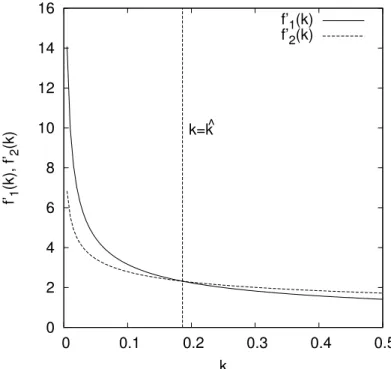
The situation described by (13) is depicted in Fig.1. Since the graphs of f₁^′(k) and f₂^′(k), both of which are negatively sloping, have only one intersection at k= ˆk, the (13) implies that technology 1 is chosen for k ≤ ˆk and technology 2 is chosen for k> ˆk.

Thus, Eqs.(10) turn into the following equation:

k_t+1 =h(k_t)=

{ h₁(k_t)= s(1−a)Ak^a_t, if 0≤ k_t ≤ ˆk,

h₂(k_t)= s(1−b)Bk^b_t, if ˆk <k_t. (14) We also find a point k^∗ >0 such that

h₁(k^∗)= h₂(k^∗), (15)

which is uniquely given by

k^∗ =

[A(1−a) B(1−b)

]1/(b−a)

. (16)

(11)

0 2 4 6 8 10 12 14 16

0 0.1 0.2 0.3 0.4 0.5

f’1(k), f’2(k)

k k=k ^

f’₁(k) f’₂(k)

Figure 1: The graphs of f₁^′(k) and f₂^′(k). They have only one intersection at k = ˆk.

A= B= 2,a= 0.5, and b= 0.7.

As ˆk

k^∗ =

[a(1−b) b(1−a)

]1/(b−a)

<1 (17)

by (12), we have ˆk <k^∗. It must be noted that h^′_i(k)>0 for k> 0, we have h^′₁(k^∗)

h^′₂(k^∗) = a

b <1. (18)

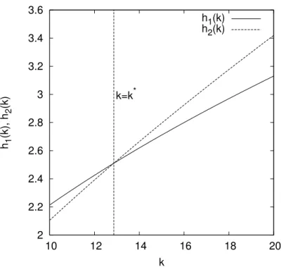
It implies that the graph of h₂(k) cuts that of h₁(k) from below at k= k^∗. This situation is depicted in Fig.2.

The graphical argument shows that if Eq.(14) has a positive steady state, then it would be globally attracting. As we are interested in non-stationary behaviors, we examine the case where Eq.(14) has no positive steady state. Let e_i > 0 be such that h_i(e_i) = e_i for i= 1,2. A simple computation shows that

e₁ =[s(1−a)A]¹^/⁽¹⁻^a) and e₂= [s(1−b)B]¹^/⁽¹⁻^b). (19) It would be suﬃcient for the following inequalities to hold to ensure that Eq.(14) does not have a positive steady state:

e₂< ˆk<e₁. (20)

(12)

2 2.2 2.4 2.6 2.8 3 3.2 3.4 3.6

10 12 14 16 18 20

h1(k), h2(k)

k k=k^*

h₁(k) h₂(k)

Figure 2: The graphs of h₁(k) and h₂(k). The graph of h₂(k) cuts that of h₁(k) from below at k =k^∗. A= B= 2,a=0.5,b= 0.7, and s= 0.7.

The following lemma shows that the set of parameter values that realize the inequalities given by (20) is not empty.

Lemma 1. Let a,b ∈ (0,1) with a < b, B > 0 and s ∈ (0,1) be given. Subsequently, there exist A > 0 and A > 0 with A < A such that the inequalities given by (20) hold for A∈(A,A).

Proof. See Appendix.

For A∈(A,A), it is evident that every trajectory generated by Eq.(14) eventually en- ters the trapping interval T = [h₂(ˆk),h₁(ˆk)] and never leaves it. Thus, in order to study the long-run behavior of the model of this situation, it is suﬃcient to focus on the dynamics of the trapping interval T .

In what follows, we assume that the parameters are taken as in Proposition 1. It must be noted that h2(ˆk) < ˆk< h1(ˆk). Let h_|T : T →T be the restriction of the mapping h to T . As h(T ) ⊂T , h_|_T is well-defined. Therefore, the goal of this study is to provide a detailed characterization of the dynamics of the mapping h_|_T : T →T .

In order to simplify the analysis of the dynamics of h_|_T, we use a variable change via a homeomorphism (i.e., a continuous, one-to-one, and onto mapping)φ: T → I = [0,1]

(13)

such that

x_t = φ(k_t)= log[

kt/s(1−b)Bˆk^b]

log b(1−a)/a(1−b) (21)

to obtain a mappingτ: I → I, which is topologically equivalent to h_|T : T → T , defined by

x_t₊₁ =τ(x_t)=

{ 1+a(x_t−c) if 0≤ x_t ≤ c,

b(xt −c) if c< xt ≤ 1, (22) where

c= c(s,A)= φ(ˆk)=

1−b

b−alog [aA/bB]−log s(1−b)B

log b(1−a)/a(1−b) . (23) Therefore, we focus on the analysis of Eq.(22) in the sequel. It must be noted that the aforementioned model turns piecewise linear through the variable change, which makes our model significantly tractable.

It is also worth noting that the graph of Eq.(22) has two branches with diﬀerent slopes, a and b, while Ishida and Yokoo (2004) and Asano et al. (2012) deal with a case of a= b.

1.3 Two types of dynamics

It is interesting to note that Eq.(22) can be identified with a simplified version of Caian- iello’s equation in the neural networks, whose original model is proposed by Caianiello to describe the behavior of a “model of brain” or “thinking machine”; this model is studied by Nagumo and Sato (1972) in detail. Additionally, Hata (2014) comprehensively analyzes this sort of equation, and we utilize results of Hata’s (2014) analysis for the mathematical neuron model to study economic growth.

When we investigate Eq.(22), the position of the threshold c(s,A) on the unit interval plays an important role. The position of the threshold characterizes the dynamical prop- erty of the model. Generally, for a given value of c, Eq.(22) has either a globally attracting periodic cycle or a non-periodic attractor. We examine the periodic case in section 1.3.1 and the non-periodic case in section 1.3.3.

First, we show that c(s,A) can take any value within the range (0,1), independently of the parameters a and b.

Lemma 2. For any a,b ∈(0,1) with a< b and for any c^∗ ∈(0,1), there exist s^∗ ∈ (0,1) and A^∗∈(A,A) such that c(s^∗,A^∗)= c^∗.

1.3.1 Periodic dynamics

All propositions in section 1.3.1 and section 1.3.3 can be almost directly⁵derived by the results of Hata (2014).

5In what follows, we provide mathematical formulae for a<b, while results of Hata’s (2014) analysis work for b<a. Thus, we need slight modifications.

(14)

The following proposition ensures the existence of a globally attracting periodic cycle in Eq.(22).

Proposition 1. For each irreducible fraction p/q ∈ (0,1), there exists a closed interval

∆(p/q) ⊂ (0,1) such that if c(s,A) ∈ ∆(p/q), for any x ∈ (0,1), then the orbit of x converges to some periodic orbit of period q.

Proof. See Hata (2014), Theorem 4.2 in p.36 and Theorem 10.1 in pp.117–118.

To be more precise, if c(s,A) ∈ ∆(p/q), then the Eq.(22) has a globally attracting cycle of period q, which visits the interval (0,c) p times and the interval (c,1) q−p times.

Later, in the study, we refer to the closed interval∆(p/q) as the periodic interval for p/q.

Subsequently, we can almost completely grasp the dynamical features of the model by verifying to which periodic interval the threshold c belongs.

Due to the piecewise linearity of the model, we can exactly calculate the left and right endpoints of the periodic interval∆(p/q) as follows. Let∆(p/q)= [L_p_,_q,R_p_,_q] and

P_p,q(w,z) =

∑q k=1

w^k−1z^⌊pk/q⌋, (24)

P⁺_p_,_q(w,z) =

∑q k=1

w^k−1z^{⌈pk/q⌉−1}, (25)

where⌊⌋and⌈⌉represent the floor and ceiling function, respectively. In other words,⌊x⌋is the largest integer that is not greater than x. On the other hand,⌈x⌉is the smallest integer that is not less than x. Subsequently, we have

L_p_,_q = 1 b

P_q_,_p(a/b,b)

P⁺_p_,_q(b,a/b), (26) R_p_,_q = 1

b

P⁺_q_,_p(a/b,b)

Pp,q(b,a/b). (27)

See Hata (2014) for more details.

Using Eq.(26) and (27), we can calculate the periodic interval for any fraction q/p∈ (0,1). Given q, we can use lemma 2 to construct the model that has an attracting cycle of period q.

Finally, we provide a few important properties of the periodic interval∆(p/q).

Proposition 2. The interval∆(p/q) has the following properties.

1. Let p/q and r/s be irreducible fraction in (0,1) with p/q < r/s. Subsequently,

∆(p/q)∩∆(r/s)= ∅and sup∆(p/q)≤inf∆(r/s).

2. ∪_p_/_q_∈_[0_,_1]_∩Q∆(p/q)=1.

Proof. See Hata (2014), Theorem 10.1 in pp.117–118 and Theorem 10.7 in p.132.

(15)

Proposition 2 states that the union of all the intervals is disjoint and its Lebesgue measure equals to 1. However, as shown later, the family of closed intervals is not a cover of the unit interval. Therefore, one might want to examine the case where the value c(s,A) does not lie in any periodic interval∆(p/q). We investigate such a case in section 1.3.3.

1.3.2 Examples

In this section, we provide a few examples for the periodic intervals. Given p = 1, we consider the cases∆(1/q) and∆((q−1)/q). Subsequently, we have

P_q_,₁(a/b,b) = (a/b)⁰b^⌊^q^⌋

= b^q, and

P⁺₁_,_q(b,a/b) =

∑q k=1

b^k⁻¹(a/b)^⌈^k^/^q^⌉−¹

=

∑q k=1

b^k⁻¹. Moreover, we have

P⁺_q,1(a/b,b) = (a/b)⁰b^⌈q⌉−1

= b^q⁻¹, and

P1,q(b,a/b) =

∑q k=1

b^k⁻¹(a/b)^⌊^k^/^q^⌋

= (a/b)⁰

q−1

∑

k=1

b^k⁻¹+(a/b)b^q⁻¹

=

q−2

∑

k=1

b^k−1+(1+a)b^q−2.

Using Eq.(26) and (27), we can derive the left and right endpoints of the interval∆(1/q) as

L1,q = b^q⁻¹

∑q

k=1b^k⁻¹, (28)

R₁_,_q = b^q−2

∑q−2

k=1b^k⁻¹+(1+a)b^q⁻². (29)

(16)

Similarly, by taking p = q−1, we can calculate the left and right endpoints of the interval∆((q−1)/q) in the following explicit forms:

L_q₋₁_,_q = 1− a^q⁻²

∑q−2

k=1a^k−1+(1+b)a^q−2, (30)

R_q₋₁_,_q = 1− a^q−1

∑q

k=1a^k⁻¹. (31)

If we further set q=3, we have

L1,3 = b²

1+b+b², (32)

R₁_,₃ = b

1+(1+a)b. (33)

Additionally, we have

L₂_,₃ = 1− a

1+(1+b)a = 1+ab

1+(1+b)a, (34)

R₂_,₃ = 1− a²

1+a+a² = 1+a

1+a+a². (35)

By letting a= 0.5 and b=0.7 and using Eq.(32) through (35), we have

∆ (1

3 )

= [L_1,3,R_1,3]≈ [0.22374,0.34146],

∆ (2

3 )

= [L₂_,₃,R₂_,₃]≈ [0.72973,0.85714].

Fig.3 (a) depicts the trajectory generated by Eq.(22) with c ∈∆(1/3) for an initial condi- tion x0 ∈(0,1). On the other hand, Fig.3 (b) depicts the case where c∈ ∆(2/3). Indeed, the trajectory of each case converges to a period-3 cycle. We can also observe that the cycle visits the interval (0,c) once within one cycle in case of (a) and twice in case of (b), depending on the numerator of 1/3 and 2/3, respectively. It must be noted that the dynamic features described above are independent of initial conditions x₀.

(17)

0 1

xt+1

x_t

∆(1/3) x_t=c(s,A)

x₀

(a) The trajectory from initial value x0for c(s,A)∈∆(1/3).

0 1

xt+1

x_t

∆(2/3) x_t=c(s,A)

x₀

(b) The trajectory from initial value x0for c(s,A)∈∆(2/3).

Figure 3: Trajectories under Eq.(22) for a = 0.5 and b = 0.7. In (a), the trajectory converges to the period-3 cycle that visits (0,c) once within one cycle. In (b), the trajectory converges to the period-3 cycle that visits (0,c) twice within one cycle.

(18)

1.3.3 Non-periodic dynamics

In this section, we discuss the non-periodic dynamics of our model.

Let

Γ = [0,1]\ ∪

p/q∈[0,1]∩Q

∆(p/q).

The setΓis the remainder obtained from the unit interval [0,1] by deleting infinite disjoint closed intervals considered in section 1.3.1.

We can show the following.

Proposition 3. For any a and b with 0< a< b< 1, the setΓis non-empty and uncount- able.

If c(s,A)∈Γ, Eq.(22) does not have any more periodic cycle. Let Ωτ =

∩∞ n=0

clτⁿ([0,1]),

where clX represents the closure of X. Subsequently, as shown in Hata (2014, Theorem 7.1 in p.76 and Theorem 8.5 in p.90),Ωτ is a compact and totally disconnected uncountable set, such as a Cantor set. Subsequently, we have the following fact:

Proposition 4. If c(s,A)∈Γ, for any x∈(0,1), then theω-limit set of x, i.e.,∩_∞

n=0∪_∞

k=nclτ^k(x), equals toΩτ.

Proof. See Hata (2014), Theorem 7.4 in p.80 and Theorem 8.5 in p.90.

We can conclude that, for c(s,A) ∈ Γ, Eq.(22) has a global non-periodic attractor; it implies that once such a threshold value is chosen, then the economy would fluctuate in a non-periodic manner in the long run for any initial condition,.

It should be noted, however, that the setΓis extremely “thin.” In fact, we can assert the following:

Proposition 5. The Hausdorﬀdimension of the setΓis zero.

Proof. See Hata (2014), Theorem 10.10 in p.139.

See, for example, Falconer (2003) for the definition of the Hausdorﬀdimension. Con- sidering the fact that the Cantor Middle Third set (with Lebesgue measure zero) has a positive Hausdorﬀdimension, while that ofΓis zero, we may say that the setΓis much sparser than the Cantor set mentioned above. It implies that our model cannot virtually reproduce the non-periodic fluctuations in the long run.

(19)

1.4 Rotation number

We introduce a useful tool for describing the dynamical behavior of our model and investigate how the parameter values aﬀect the dynamics of the model. In what follows, we represent Eq.(22) asτa,b to emphasize the parameter dependence. For any x ∈(0,1), we define

ϵ(x)=

0 (x∈[0,c)), 1 (x∈[c,1]). Moreover, we also define

ϵk(x)= ϵ◦τ^ka,b(x). It is known that, for anyτa,b, the limit

ρ(τa,b)= lim

n→∞

1 n

∑n−1 k=0

ϵk(x)

exists and is independent of the choice of x ∈ (0,1). See, for example, Hata (2014), Theorem 3.2 in pp.23-24. The valueρ(τa,b) is called the rotation number⁶ofτa,b. Clearly, if c(s,A)∈∆(p/q), then the rotation number equals to p/q. On the other hand, if c(s,A)∈ Γ, then the rotation number is irrational.

As expected, for the given a and b, we examine the relationship between theρ(τa,b) and the value c, and eventually examine the parameter values s and A. In what follows, we regard the rotation number as a function of c(s,A). In this sense, we define

Ra,b(c(s,A))= ρ(τa,b).

It is known that Ra,b(c(s,A)) is continuous with respect to c, and its derivative exists and vanishes almost everywhere. See Hata (2014), Theorem 10.11 in p.140. Taking the con- tinuity and the result of Proposition 2 into account, we can see that R_a_,_b(c) is monoton- ically increasing with respect to the threshold c. Now, we examine the relationship of the threshold c and the parameters s and A. Since c(s,A) is continuous with respect to s and A, R_a_,_b(c(s,A)) is also continuous with respect to s and A. Moreover, since c(s,A) is monotonically decreasing with respect to s and increasing with respet to A, we have the following proposition.

Proposition 6. The rotation number function Ra,b(c(s,A)) is continuous and monotoni- cally decreasing with respect to s and monotonically increasing with respect to A. More- over, the partial derivatives of R_a,b(c(s,A)) exist and vanish almost everywhere.

6The term rotation number seems odd in this context. This is a terminology originally used in the dynamical systems theory to characterize the rotating dynamics of a homeomorphism on the circle. The same concept is referred to in diﬀerent ways, depending on the contexts, such as the expansion rate in Ishida and Yokoo (2004) and the average firing rate in the neuron context (Nagumo and Sato, 1972).

(20)

0.2 0.3 0.4 0.5 0.6 0.7 0.8 0.9 1

0.4 0.5 0.6 0.7 0.8 0.9 1 Ra,b(c(s,A))

S

(a) The graph of rotation number function R_a_,_b(c(s,A)) with respect to s.

0 0.1 0.2 0.3 0.4 0.5 0.6 0.7 0.8 0.9 1

1.4 1.6 1.8 2 2.2 2.4 2.6 2.8 Ra,b(c(s,A))

A

(b) The graph of rotation number function Ra,b(c(s,A)) with respect to A.

Figure 4: The devil’s staircases: the graphs of the rotation number function R_a_,_b(c(s,A)) for a =0.5,b=0.7, and B= 2. (a) A=2.2. (b) s =0.7.

(21)

Fig.4 (a) and (b) depict the graph of R_a_,_b(c(s,A)) with respect to s and A, respectively.

Fig.4 may invoke the well-known Cantor’s function. However, contrary to the Cantor’s function, the rotation number function is not H¨older continuous for any order. In other words, for any C, α∈R+, there exist x,y∈(0,1) such that|R_a_,_b(x)−R_a_,_b(y)|>C|x−y|^α.⁷ In this sense, the rotation number function discussed here should be distinguished from the Cantor’s function.

Finally, we present our remarks on the rotation number. In Fig.4, we can see the rotation number 2/5 between the rotation numbers 1/2 and 1/3. It is clear that the mediant (1+1)/(2+3) implies the number 2/5. This is reminiscent of the construction of the Farey sequence in the number theory.⁸ The following proposition immediately follows from the continuity and monotonicity of the rotation number function.

Proposition 7. For any two rotation numbers, p/q < r/s, there is a rotation number of the form (p+r)/(q+s) between p/q and r/s.

Precisely, if R_a_,_b(c₁) = p/q and R_a_,_b(c₂) = r/s, then there would exist c^∗ ∈ (c₁,c₂) such that R_a,b(c^∗) = (p+r)/(q+ s). Let u/v be the irreducible form of (p+ r)/(q+ s).

Subsequently, proposition 7 says that if an attracting period-q cycle and an attracting period-s cycle are detected for some thresholds c₁ and c₂, respectively, then one will find another attracting period-v cycle between them that would visit u times the interval (0,c^∗), corresponding to the regime of technology 1, and v−u times the interval (c^∗,1), corresponding to the regime of technology 2.

Remark 1. Here, we briefly discuss the mechanism that generates periodic cycles and attempt to provide insight into the economic intuition behind the model.

Fig.5 shows the time series obtained from the model with rotation number 6/7. At a low level of capital stock, technology 1, which is characterized by (A,a), yields a higher rate of return to capital than that obtained from technology 2, characterized by (B,b).

Therefore, for an initially low capital stock, the owner of the firm chooses technology 1 and the capital stock increases, as in the case of the traditional OLG model with no technology choice. On the other hand, if the capital stock exceeds some level, technology 2 provides a higher rate of return to capital than that of technology 1. As a result, the owner switches technology 1 to technology 2.

However, it should be noted that a high rate of return to capital does not necessarily imply a high level of wage, nor eventually the amount of saving. Indeed, when the owner changes technology (see box A in Fig.5), the wage rate drops down, which induces a decrease in capital stock in the next period. Subsequently, if the decrease in capital stock is suﬃcient, the owner will switch back to technology 1. Hence, the story repeats, and the capital stock in the economy exhibits periodic cycles.

For rotation numbers that are not of ¹_n or ⁿ⁻¹_n , persistent fluctuations also occur in the same way. However, the switches of technology will occur more frequently in such a case.

7See, for example, Lawrence (1998).

8See, for example, Hardy and Wright (1979) for the Farey sequence.

(22)

1 2 3 4 5 6 7 8 9 10 11 12 13 14 15 Time : t

A

k_t w_t r_t¹ r_t²

Figure 5: The time series of capital stock k_t, wage rate w_t, and two rates of return to capital, denoted by r¹_t and r_t² for technology 1 and 2, respectively, for rotation number 6/7.

1.5 Concluding remarks

We have developed a tractable endogenous growth cycle model that is described by a piecewise linear diﬀerence equation. Nonlinearity generating perpetual fluctuations are attributed to the choice of technology. Despite the simplicity of the model, its dynamics are rich enough to generate a cycle of any arbitrarily large period. Moreover, owing to the results from the study of mathematical neuron models, we can completely specify the set of parameters for which a specific type of periodic cycle appears. It is also interesting that our purely economic model can be linked with the mathematical “brain,” or neuron, model as well as to the number theory.

We have also shown that the model can exhibit non-periodic behavior for a non-empty and uncountable set of parameters. Nonetheless, such a set of parameters is extremely thin, and hence the non-periodic perpetual fluctuations in the long run are relatively patho- logical in our model. In other words, our model is virtually incapable of reproducing economic fluctuations that are considered recurrent but not periodic in nature.

However, there might be several ways of extending the model in this study to repro- duce non-periodic perpetual fluctuations, such as the chaotic behavior. For instance, it is

(23)

possible to smooth the discontinuous map in our model by introducing the “mispercep- tion” idea of Yokoo and Ishida (2008) and Asano and Yokoo (2019) and thus to determine if the modified model can exhibit chaos as a typical phenomenon. Alternatively, it would also be interesting to introduce a continuum of technologies through which the model might be smoothed without losing strong nonlinearity. These areas could serve as the focus of future research. We hope that the simple model presented here may be used as a building block for other potential endogenous growth cycle or business cycle models in more complex settings.

1.6 Appendix

1.6.1 Proof of Lemma 1

Proof. By arranging e2 < ˆk and ˆk < e1 for A, we have A < A and A < A, respectively, where

A=m^b−a₁ B(1−a)/(1−b) and A=m(b−a)(1−a)/(1−b)

2 B(1−a)/(1−b) (A.1)

with

m₁ =[s(1−b)]^1/(1−b)(b/a)^1/(b−a) and m₂= [s(1−a)]^1/(1−a)(b/a)^1/(b−a). (A.2) It remains to show that m1 < m⁽¹₂⁻^a)^/⁽¹⁻^b). Suppose that this is not the case. Subsequently, we have m₁ ≥m⁽¹₂⁻^a)^/⁽¹⁻^b), or

[s(1−b)]¹^/⁽¹⁻^b)(b/a)^1/(b−a) ≥[s(1−a)]^1/(1−b)(b/a)(1−a)/[(b−a)(1−b)], (A.3) implying that

1−b 1−a ≥ b

a, (A.4)

or a ≥b, which is a contradition.

1.6.2 Proof of Lemma 2

Proof. Taking (A.1) and (A.2) of Appendix A into account, a simple calculation shows that, for any s ∈ (0,1), c(s,A) = 0 and c(s,A) = 1. By the continuity of c(s,A) with respect to A, for any s^∗ ∈(0,1) and c^∗ ∈(0,1), there exist A^∗∈(A,A) such that c(s^∗,A^∗)=

c^∗.

1.6.3 Proof of Proposition 3

Proof. The proposition follows from the fact that the closed interval [0,1] cannot be partitioned (in the sense of set theory) into a countably infinite number of non-empty closed intervals. See Sierpi´nski (1918) or other mathematical textbooks of topology for more details.

(24)

The above fact implies that the union of periodic intervals,∪

p/q∈[0,1]∩Q∆(p/q), is not a cover for the closed interval [0,1]. Therefore, the set Γ = [0,1]\∪

p/q∈[0,1]∩Q∆(p/q) is non-empty. Now, suppose that the setΓis countable. For each x∈Γ, let{x}be a singleton set. Subsequently, the union of the set of periodic intervals and the set of {x}becomes countable and gives a partition of the closed interval [0,1], which contradicts the above

fact. Thus, the setΓis uncountable.

(25)

2 Complex Dynamics of an Inflation Model with a Piece- wise Linear Phillips Curve

2.1 Introduction

In this study, we construct a simple inflation-unemployment model exhibiting complex behaviors of macroeconomic variables. The model is composed by simple macroeconomic relations such as the expectations-augmented Phillips curve, static expectations, and a dynamic version of Okun’s law, all of which can be found in undergraduate macroeconomic textbooks such as Blanchard (1997).

In addition to these traditional relations, we assume that the incorporated Phillips curve is piecewise linear for the purpose of introducing slight nonlinearity into the model with all other relations being linear. The nonlinearity of the Phillips curve in a macroeconomic model can aﬀect the qualitative features of its dynamics. The topic of nonlinearity has a long history in the literature; however, little attention has been paid to nonlinear dynamics from the viewpoint of the Phillips curve, leaving a dearth of analytical research to this eﬀect. Few exceptions include Soliman (1996a, 1996b) and Chiarella, Flaschel, Gong, and Semmler (2003). Chiarella et al. (2003) introduce a kinked Phillips curve into a Keynesian monetary macroeconomic model to demonstrate the complex dynamics in the model using numerical analysis. Soliman (1996a, 1996b) develop similar inflation model to ours. He introduces a smooth nonlinear Phillips curve, and suggests that the model generates chaotic dynamics using computer simulations.

Adopting piecewise linearity to the Phillips curve has a distinct advantage over other types of nonlinearities. In fact, we show in the sequel that the piecewise linearity of the Phillips curve allows us to derive certain exact analytical results using a direct calculation, which otherwise could not be obtained when the Phillips curve is assumed to have smooth nonlinearity. For instance, our two-dimensional model is rigorously shown to have a transverse homoclinic point (explained in Section 2.3), which implies the existence of a horseshoe, that is, a chaotic invariant set. However, the same could hardly be shown for the Soliman’s model, which is equipped with a specific smooth Phillips curve, without relying on numerical methods.

It is worth emphasizing here that establishing the existence of chaos in a higher- dimensional model is not impossible but diﬃcult without computer assistance, even when the model is completely specified. In fact, the economic literature contains few higher- dimensional economic models that are analytically established to be chaotic. See Yokoo (2000) and Chen and Ming (2008) for OLG models; Onozaki, Sieg, and Yokoo (2003) for a cobweb model; Brock and Hommes (1997) for the heterogeneous belief model;

and Droste, Hommes, and Tuinstra (2002) for a Cournot-type duopoly with heterogeneous belief. These economic models are established, in a certain sense, as chaotic when the systems are two dimensional but close to a one dimensional. However, owing to piecewise linearity, we can show that, without relying on numerical methods, our model exhibits chaos as well as other nonlinear phenomena, including coexisting periodic attrac-