Anomalous random walks and diffusions:
From fractals to random media
By
Takashi KUMAGAI
July 2014
R
ESEARCH
I
NSTITUTE FOR
M
ATHEMATICAL
S
CIENCES
From fractals to random media
Takashi Kumagai
⇤Abstract. We present results concerning the behavior of random walks and di↵usions on disordered media. Examples treated include fractals and various models of random graphs, such as percolation clusters, trees generated by branching processes, Erd˝os-R´enyi random graphs and uniform spanning trees. As a consequence of the inhomogeneity of the underlying spaces, we observe anomalous behavior of the corresponding random walks and di↵usions. In this regard, our main interests are in estimating the long time behavior of the heat kernel and in obtaining a scaling limit of the random walk. We will overview the research in these areas chronologically, and describe how the techniques have developed from those introduced for exactly self-similar fractals to the more robust arguments required for random graphs.
Mathematics Subject Classification (2010). Primary 60J45; Secondary 05C81, 60K37.
Keywords. Fractals, heat kernel estimates, percolation, random media, sub-di↵usivity
1. Introduction
Since the mid-sixties, mathematical physicists have investigated anomalous behav-ior of random walks and di↵usions on disordered media (see for example [17]). The random walk on a percolation cluster – the so-called ‘ant in the labyrinth’ ([24]) – is one of the central examples. Recall that the bond percolation model on the lattice Zd, d 2, is defined as follows: each nearest neighbor bond is open with
probabil-ity p 2 [0, 1] and closed otherwise, independently of all the others. It is well-known that this model exhibits a phase transition, whereby if ✓(p) := Pp(|C(0)| = +1),
where C(0) is the open cluster containing 0, then there exists pc = pc(Zd) 2 (0, 1)
such that ✓(p) = 0 if p < pc and ✓(p) > 0 if p > pc. For p > pc, there exists
a unique open infinite cluster upon which the long time behavior of the simple random walk is similar to that of the simple random walk onZd (see Section 4.1).
For the simple random walk on the critical percolation cluster, however, in 1982 Alexander and Orbach [1] made a striking conjecture about how there might be quite di↵erent behavior. (To make the problem mathematically precise, one has to consider the critical percolation cluster conditioned to be infinite, as we discuss in
Section 4.2.) Let Y = {Y!
n}n2Nbe the simple random walk on the cluster (i.e. Yn!
is in one of the adjacent neighbors of Y!
n 1with equal probabilities), and p!n(x, y)
be its heat kernel (transition density); see (3.3) for precise definition. Here and in the following, the suffix ! stands for the randomness of the media. Define
ds:= 2 lim n!1
log p! 2n(x, x)
log n (1.1)
as the spectral dimension of the cluster if the limit exists. (To be precise, the original definition of ds was the ‘density of states’, which gives the asymptotic
growth of the eigenvalue counting function.) One formulation of the Alexander-Orbach conjecture is that ds= 4/3 for all d 2. Clearly, this expresses anomalous
behavior for the random walk, since ds= d for simple random walk onZd. These
works stimulated a lot of interest from mathematical physicists in exact fractals as well (see for example [41]).
Mathematical progress on these problems started to be made in the late eighties. In 1986, Kesten wrote two beautiful papers ([31, 32]) in which he constructed an ‘incipient infinite cluster’ for critical percolation on Z2 and showed that the random walk on this was anomalous (in the latter work, he also considered random walks on critical models of trees); these were the first significant mathematically rigorous works in this area. Kesten’s work and mathematical physicists’ work mentioned above triggered intensive research on di↵usions on fractals, which are “ideal” disordered media. As part of this, Brownian motion was constructed on typical fractals, such as the Sierpinski gasket, and properties of these processes were obtained (see Section 2). These included detailed heat kernel estimates of the so-called sub-Gaussian form, meaning that the heat kernel is bounded from above and below by c1t ds/2exp ⇣ c2 ⇣ d(x, y)dw t ⌘1/(dw 1)⌘
with di↵erent pairs of constants (c1, c2) for the upper and lower bounds. Here
dw> 2 is a constant and d(·, ·) is a geodesic distance on the fractal.
While di↵usions on fractals had been extensively studied by 2000 and continue to be actively studied, the turn of the century saw increasing moves being made to analyze “fractal-like spaces” instead of working only on ideal fractals. The key issue here is whether the sub-Gaussian estimates mentioned above are stable under perturbations of spaces and operators. (Note that when ds= d and dw = 2, the
corresponding estimates are Gaussian estimates, and such a perturbation theory was extensively developed in the nineties.) In this direction, several functional inequalities have been shown to be equivalent to the sub-Gaussian estimates, some of which are stable under perturbations, meaning that the stability problem has been affirmatively resolved (see Section 3).
It turns out that such a stability theory is useful even for the analysis on ran-dom media, including percolation clusters as Kesten considered. Indeed, some functional inequalities have been modified and applied to random walks on var-ious models of disordered media, especially on percolation clusters (see Section 4). Specifically, the Alexander-Orbach conjecture has been affirmatively solved for
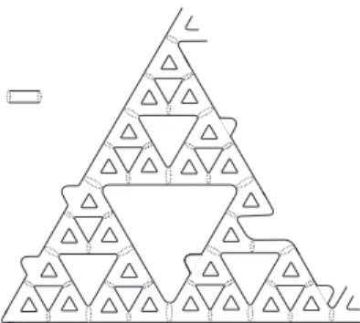
Figure 1. Sierpinski gasket graph V0 and Sierpinski gasket ˆK
high dimensions (Theorem 4.4). For some models, scaling limits of random walks have also been established (see Section 4.1 and Section 5); these include supercrit-ical percolation clusters, critsupercrit-ical branching processes conditioned to be large, the Erd˝os-R´enyi random graph in the critical window, and the 2-dimensional uniform spanning tree.
The aim of this paper is to give a overview of the stream of research introduced above. It is a very restricted survey and the references are far from complete. Due to space restriction, for papers which are very important but for which details are not discussed in this paper, names of authors and years of publication are mentioned but without inclusion in the list of references. We apologize to the authors of relevant papers which are not cited here. Readers can find more detailed information in the following books/surveys [5, 7, 17, 19, 23, 25, 27, 29, 33, 34, 36, 38, 39, 42, 44, 45].
Notation. We write f ⇣ g if there exist constants c1, c2> 0 such that c1g(x)
f (x) c2g(x) for all x, and f ⇠ g if lim|x|!1f (x)/g(x) = 1.
2. Anomalous heat transfer on fractals
Let a = (0, 0), b = (1, 0), c = (1/2,p3/2), and set
F1(x) = (x a)/2 + a, F2(x) = (x b)/2 + b and F3(x) = (x c)/2 + c.
Then, there exists unique non-void compact set such that K = [3
i=1Fi(K); we call
K the 2-dimensional Sierpinski gasket. Define the unbounded Sierpinski gasket as ˆ
K = [1 n=02nK.
We first explain the construction of Brownian motion on ˆK. Let V0= 1 [ m=0 2m⇣ 3 [ i1,··· ,im=1 Fi1 · · · Fim({a, b, c}) ⌘ , Vm= 2 mV0.
The closure of [m 0Vm is ˆK. Let {X(i)}i 0 be the simple random walk on V0.
of X(i) in V0(i.e. points in the same triangles with length 1 as those X(i) belongs
to) with equal probabilities. Let Xm(i) := 2 mX(i) be the simple random walk on
Vm. Since Xmmoves distance 2 m per unit time, Xm(i) ! 0 as m ! 1 for fixed
i. So, we must speed up the random walks in order to obtain a non-trivial limit. It is plausible to choose the time scale as the average time for the random walk on Vm+1 starting from a point in Vm to reach one of the neighboring points in Vm.
By the self-similarity and symmetry of ˆK, this average time is independent of m and it is equal to the average time for X1starting from a to arrive at either b or c.
A simple calculation deduces that the value is 5. Let Yt(m):= Xm([5mt]). Then,
it can be proved that {Y(m)} converges to a non-trivial di↵usion on ˆK as m ! 1,
which is called Brownian motion on ˆK. (One can construct Brownian motion on K similarly.) Brownian motion on the gasket was first constructed by Goldstein (1987) and Kusuoka (1987) independently. Characterization of Brownian motion is also known; any self-similar di↵usion process on ˆK whose law is invariant under local translations and reflections on each small triangle is a constant time change of this di↵usion ([16]).
The corresponding Laplacian is defined as follows: f (x) = lim m!15 m⇣ X xi: x⇠xm i f (xi) 4f (x) ⌘ , x 2 [m 0Vm\ {0},
for f in a suitable function space, where x ⇠ y means that x and y are adja-m cent in Vm. Note that the standard approximation for the Laplacian on R is
f (x) = limm!122m(f (x + 2 m) + f (x 2 m) 2f (x)) for f 2 C2(R). Set
dw= log 5/ log 2 so that 5 = 2dw. Naively, we can say that the Laplacian on the
gasket is a “di↵erential operator of order dw”. (One way of stating this
rigor-ously is that the domain of the corresponding Dirichlet form on the gasket is a Besov space of order dw/2 (Jonsson (1996), Grigor’yan-Hu-Lau (2003)).) Kigami
(1989) was the first to construct the Laplacian on the gasket directly. It turns out that the theory of Dirichlet forms ([23]) is well-applicable to this area, and di↵u-sions (self-adjoint operators) on fractals have been constructed through Dirichlet forms systematically. Fukushima-Shima (1992) is one of the first who applied the Dirichlet form theory to fractals.
OnRd, we can define ˆK similarly from the family of (d+1)-th contraction maps
with contraction rate 1/2. (For d = 1, ˆK = [0, 1).) The Hausdor↵ dimension of the d-dimensional gasket is df = log(d + 1)/ log 2. The time scaling is d + 3 and
dw= log(d + 3)/ log 2.
In order to understand the asymptotic properties of the process, it is very important and useful to obtain detailed heat kernel estimates. Let {B(t)}t 0 be
Brownian motion on the gasket and define Ptf (x) = Ex[f (B(t))] =
Z
ˆ K
pt(x, y)f (y)µ(dy),
where µ is the normalized Hausdor↵ measure on ˆK. {Pt}t 0is the semigroup and
is a fundamental solution of the heat equation for the Laplacian. For the case of Brownian motion onRd, p
t(x, y) is the Gauss-kernel (2⇡t)1d/2exp( |x y|2/(2t)). Let d(x, y) be the shortest distance between x and y in ˆK. The following sub-Gaussian heat kernel estimates are obtained by Barlow-Perkins [16].
Theorem 2.1. pt(x, y) obeys the following estimates for t > 0, x, y 2 ˆK:
c1t df/dwexp ⇣ c2 ⇣ d(x, y)dw t ⌘1/(dw 1)⌘ pt(x, y) c3t df/dwexp ⇣ c4 ⇣ d(x, y)dw t ⌘1/(dw 1)⌘ . (2.1)
The simple random walk on V0also obeys (2.1) for d(x, y) t 2 N (Jones (1996)).
From the probabilistic viewpoint, dw is the order of the di↵usion speed of
par-ticles and it is called the walk dimension. Indeed, by integrating (2.1), we have c5t1/dw Ex[d(x, B(t))] c6t1/dw. As dw > 2, the behavior of the process is
anomalous (for a long time, it di↵uses slower than Brownian motion onRd, so the
behavior is sub-di↵usive). This di↵usion does not have finite quadratic variation, so it is not a semi-martingale ([16]). Its martingale dimension is 1 (Kusuoka (1989), Hino (2008)). Set ds/2 = df/dw. This ds, which is the same exponent as in (1.1),
gives the asymptotic growth of the eigenvalue counting function for the Laplacian on K, and it is called the spectral dimension. Spectral properties of the Laplacian have been extensively studied (Fukushima-Shima (1992), Kigami-Lapidus (1993), Barlow-Kigami (1997), Teplyaev (1998), etc.). Unlike the Euclidean case, Brown-ian motion and the LaplacBrown-ian on the gasket exhibit oscillations in their asymptotics; in the asymptotics of the eigenvalue counting function (Barlow-Kigami (1997)), in the on-diagonal heat kernel asymptotics (Grabner-Woess (1997), Kajino (2013)), and in Schilder’s large-deviation principle (Ben Arous-Kumagai (2000)).
(2.1) is a very useful estimate. Various properties of Brownian motion such as laws of the iterated logarithm can be deduced from this estimate. It also implies nice regularity properties of caloric functions u(t, x) (i.e. solutions of the heat equation @u
@t = u). For S, R 2 (0, 1), x02 ˆK, set
Q = (S + Rdw, S + 2Rdw) ⇥ B(x
0, R), Q+= (S + 3Rdw, S + 4Rdw) ⇥ B(x0, R).
The parabolic Harnack inequalities compare the values of caloric functions on Q and Q+uniformly. They imply uniform H¨older continuity of the caloric functions.
Theorem 2.2 (Generalized parabolic Harnack inequalities and H¨older continuity). There exist c1, c2, ✓ > 0 such that, for any S, R 2 (0, 1), x0 2 ˆK, if u is a
non-negative caloric function on (S, S + 4Rdw) ⇥ B(x
0, 2R), then the following hold:
sup (t,x)2Q u(t, x) c 1 inf (t,x)2Q+ u(t, x), (P HI(dw)) |u(s, x) u(s0, x0)| c2 ✓ |s s0|1/dw+ d(x, x0) R ◆✓ kuk1, (2.2) for any (s, x), (s0, x0) 2 (S + Rdw, S + 4Rdw) ⇥ B(x 0, R).
Figure 2. Penta-kun and Sierpinski carpet
In fact, (2.1) and (PHI(dw)) are equivalent under a suitable volume growth
condition as we will see in the next section. (PHI(dw)) implies various regularity
properties of harmonic functions such as the elliptic Harnack inequalities and the Liouville property (i.e. if u is a non-negative harmonic function on ˆK, then u is a constant function).
For more general fractals such as nested fractals introduced by Lindstrøm (1990) and Sierpinski carpets (see Figure 2, the left figure is an example of nested fractals), Brownian motion is constructed and it is known that the heat ker-nels obey the sub-Gaussian estimates (2.1) (Barlow-Bass (1989, 1999), Lindstrøm (1990), Kumagai (1993), Fitzsimmons-Hambly-Kumagai (1994)). Characteriza-tion of Brownian moCharacteriza-tion on the fractals are also known (Metz (1996), Sabot (1997), Barlow-Bass-Kumagai-Teplyaev (2010)).
Open problem I: The existing construction of Brownian motion on the carpet requires detailed uniform control of harmonic functions (such as uniform Harnack inequalities) for the approximating processes; see for example [7]. Construct Brow-nian motion on the carpet without such detailed information.
We refer to [5, 7, 33, 34, 38, 44] for details on di↵usions/analysis on fractals.
3. Stability of parabolic Harnack inequalities and
sub-Gaussian heat kernel estimates
Since fractals are “ideal” objects in that they have exact self-similarity, it is natural to ask if the inequalities (2.1) and (PHI(dw)) are stable under perturbations of the
state space and the operator.
Let us first briefly overview the history for the case of dw = 2. For any
di-vergence operator L = Pdi,j=1@x@i(aij(x)
@
@xj) onR
d satisfying a uniform elliptic
condition, Aronson (1967) proved (2.1) with df = d and dw= 2. Later in the last
century, there are outstanding results from the field of global analysis on manifolds. Let be the Laplace-Beltrami operator on a complete Riemannian manifold M with the Riemannian metric d(·, ·) and with the Riemannian measure µ. Li-Yau
(1986) proved the remarkable fact that if M has non-negative Ricci curvature, then the heat kernel pt(x, y) satisfies
c1 (x, c2d(x, y), t) pt(x, y) c3 (x, c4d(x, y), t), (3.1)
where (x, r, t) = µ(B(x, t1/2)) 1exp( r2/t). A few years later, Grigor’yan (1991)
and Salo↵-Coste (1992) refined the result and proved, in conjunction with the re-sults by Fabes-Stroock (1986) and Kusuoka-Stroock (1987), that (3.1) is equivalent to a volume doubling condition (VD) plus Poincar´e inequalities (PI(2)) –see Def-inition 3.1 and 3.3 for defDef-initions in the graph setting. Their results were later extended to the framework of Dirichlet forms by Sturm (1996) and graphs by Del-motte (1999). Detailed heat kernel estimates are strongly related to the control of harmonic functions. The origin of ideas and techniques used in this field goes back to De Giorgi (1957), Nash (1958), Moser (1961,1964) and there are many other significant works in this area. See for example [25, 42] and the references therein. Summarizing, the following equivalence holds:
(3.1) , (VD) + (PI(2)) , (PHI(2)). (3.2) Since (VD) and (PI(2)) are stable under some perturbations, we see that (3.1) and (PHI(2)) are also stable under the perturbations.
We will discuss the extension of (3.2) to the dw > 2 case. Though such a
generalization has also been established under a metric measure space with a local regular Dirichlet form, for simplicity, we will restrict our attention to the graph setting. We first set up notation and definitions.
3.1. Setting.
Let G be a countably infinite set, and E a subset of {{x, y} 2 G ⇥ G : x 6= y}. We write x ⇠ y if {x, y} 2 E. A graph is a pair (G, E) and the graph distance d(x, y) for x, y 2 G is the length of the shortest path from x to y (we set d(x, x) = 0). We assume the graph is connected (i.e. d(x, y) < 1 for all x, y 2 G) and locally finite (i.e. |{y 2 G : {x, y} 2 E}| < 1 for all x 2 G). For x 2 G and r 0, denote B(x, r) = {y 2 G : d(x, y) r}.Now assume that the graph G is endowed with a weight (conductance) µxy,
which is a symmetric nonnegative function on G ⇥ G such that µxy > 0 if and
only if x ⇠ y. We call the pair (G, µ) a weighted graph. We can regard it as an electrical network. We define a quadratic form on (G, µ) as follows. Set
E(f, g) = 12 X x,y2G
x⇠y
(f (x) f (y))(g(x) g(y))µxy for all f, g 2 RG.
For each x 2 G, let µx=Py2Gµxy and for each A ⇢ G, set µ(A) =Px2Aµx.
µ is a measure on G. Let {Yn}n 0 be the discrete time Markov chain whose
transition probabilities are given by P (Yn+1= y|Yn= x) =
µxy
µx
Y is is called a simple random walk when µxy = 1 whenever x ⇠ y. The heat
kernel of {Yn}n 0can be written as
pn(x, y) := Px(Yn = y)/µy for all x, y 2 G, (3.3)
where we set Px(·) := P (·|Y
0 = x). Clearly, pn(x, y) = pn(y, x). We sometimes
consider a continuous time Markov chain {Yt}t 0with respect to µ which is defined
as follows: each particle stays at a point, say x for (independent) exponential time with parameter 1, and then jumps to another point, say y with probability P (x, y). The heat kernel for the continuous time Markov chain can be expressed as follows.
pt(x, y) = Px(Yt= y)/µy= 1 X n=0 e tt n n!pn(x, y) for all x, y 2 G. The discrete Laplacian corresponding to {Yt}t 0is
Lf(x) =X y2G y⇠x P (x, y)f (y) f (x) = 1 µx X y2G y⇠x ⇣ f (y) f (x)⌘µxy.
In this section, we assume the following condition on the weighted graph. Definition 3.1. Let (G, µ) be a weighted graph.
(i) We say (G, µ) has controlled weights if there exists p0> 0 such that
P (x, y) = µxy/µx p0 for all x ⇠ y 2 G.
(ii) We say (G, µ) satisfies a volume doubling condition (VD) if there exists c1> 1
such that
µ(B(x, 2R)) c1µ(B(x, R)) for all x 2 G, R 1. (3.4)
3.2. Stability.
We first introduce two types of perturbations.Definition 3.2. Let (G1, µ1), (G2, µ2) be weighted graphs with controlled weights.
(i) We say (G2, µ2) is a bounded perturbation of (G1, µ1) if G1 = G2 and there
exist c1, c2> 0 such that c1(µ1)xy (µ2)xy c2(µ1)xy for all x ⇠ y.
(ii) A map T : G1! G2is called a rough isometry if there exist positive constants
c1, · · · , c4> 0 such that the following holds for all x, y 2 G1 and y02 G2.
c11d1(x, y) c2 d2(T (x), T (y)) c1d1(x, y) + c2
d2(T (G1), y0) c3, c41(µ1)x (µ2)T (x) c4(µ1)x.
where di(·, ·) is the the graph distance of (Gi, µi), for i = 1, 2. (G1, µ1), (G2, µ2)
are said to be rough isometric if there is a rough isometry between them.
The notion of rough isometry was first introduced by Kanai (1985). Note that rough isometry corresponds to (coarse) quasi-isometry in the field of geometric group theory, which was introduced by Gromov (1981).
Definition 3.3. Let (G, µ) be a weighted graph with controlled weights and let > 1.
(i) We say (G, µ) satisfies sub-Gaussian heat kernel estimates (HK( )) if there exist c1, · · · , c4> 0 such that for x, y 2 G, n d(x, y) _ 1, the following holds:
pn(x, y) c1 µ(B(x, n1/ ))exp ⇣ c2 ⇣ d(x, y) n ⌘1/( 1)⌘ , pn(x, y) + pn+1(x, y) c3 µ(B(x, n1/ ))exp ⇣ c4 ⇣ d(x, y) n ⌘1/( 1)⌘ . (ii) We say (G, µ) satisfies (PI( )), a scaled Poincar´e inequality with exponent , if there exists a constant c1 > 0 such that for any ball BR := B(x0, R) ⇢ G with
x02 G, R 1 and f : BR! R, X x2BR (f (x) f¯BR) 2µ x c1R X x2BR (f, f )(x). Here ¯fBR:= µ(BR) 1P
y2BRf (y)µy, and (f, f )(x) := P
y⇠x(f (x) f (y))2µxy.
(iii) We say (G, µ) satisfies (CSA( )), a cut-o↵ Sobolev inequality in annuli with exponent , if there exist a constant c1 > 0 such that for every x0 2 G, R, r 1,
there exists a cut-o↵ function ' satisfying the following properties: (a) '(x) = 1 if x 2 BR, '(x) = 0 if x 2 BR+rc .
(b) Let U = BR+r\ BR. For any f : U ! R,
X x2U f (x)2 (', ')(x) c1 ⇣ X x2U '(x)2 (f, f )(x) + r X x2U f (x)2µx ⌘ . Theorem 3.4 ([2, 8, 9]). Let (G, µ) be a weighted graph with controlled weights. Then,
(VD) + (PI( )) + (CSA( )) , (PHI( )) , (HK( )). (3.5) Here and in the following, (PHI( )) means the discrete version of (PHI(dw)) in
Theorem 2.2 with dw= .
Remark 3.5. (i) There are various other equivalent conditions to (3.5); see [26, 45] and references therein.
(ii) When one of (thus all) the above conditions holds, then it turns out that 2. (iii) (CSA(2)) always holds in the graph context. (Take '(x) = 1^r 1d(x, Bc
R+r).)
Thus Theorem 3.4 is an extension of (3.2) to the cases of > 2 for graphs. (iv) The main theorem in [2] is the equivalence of the upper bound of (HK( )) and (CSA( )) plus the Faber-Krahn inequality with exponent . The results are stated on metric measure spaces.
For the = 2 case, there is a well-known method called Moser’s iteration to deduce the Harnack inequality in (3.2). In order for the method to work, it is necessary that the correct order can be deduced using linear cut-o↵ functions. If
Figure 3. Fractal-like manifold
we adopt similar arguments using the Lipschitz cut-o↵ functions for the > 2 case, then the estimates obtained are not sharp enough to establish the Harnack inequality. Roughly speaking, (CSA( )) guarantees the existence of nice cut-o↵ functions ' that satisfy E(', ') c1R µ(BR). (Note that the order of the energy
for the Lipschitz continuous cut-o↵ function is R 2µ(B
R).) The idea of the proof
of the Harnack inequality when > 2 is to apply Moser’s iteration for weighted measures ⌫x:= µx+ R (', ')(x) using (CSA( )).
Clearly, (VD), (PI( )) and (CSA( )) are stable under bounded perturbations. Further, it can be proved that they are stable under rough isometry (Hambly-Kumagai (2004)). We thus obtain the stability of (PHI( )) and (HK( )).
As mentioned above, Theorem 3.4 holds in the framework of metric measure spaces with local regular Dirichlet forms (especially Riemannian manifolds). It also holds when the walk dimension is di↵erent for short times and long times. Figure 3 is a 2-dimensional Riemannian manifold whose global structure is like that of the gasket. This can be constructed from the left of Figure 1 by changing each bond to a cylinder and putting projections and dents locally. The di↵usion corresponding to the Dirichlet form moves on the surfaces of the cylinders. Using the generalization of Theorem 3.4, one can show that any divergence operator L = P2i,j=1
@
@xi(aij(x)
@
@xj) on the manifold which satisfies the uniform elliptic condition obeys (PHI(2)) for R 1 and (PHI(log 5/ log 2)) for R 1.
3.3. Strongly recurrent case.
The problem with Theorem 3.4 is that it is in general very difficult to check (CSA( )). Under a stronger volume growth condition, a simpler equivalent condition is known.For each x 6= y 2 G, define the e↵ective resistance between them by Re↵(x, y) 1= inf
n
E(f, f) : f(x) = 1, f(y) = 0, f 2 RGo. (3.6) We define Re↵(x, x) = 0 for x 2 G.
Definition 3.6. (i) We say (G, µ) satisfies the volume growth condition (VG( )) if there exist K > 1, c1> 0 with log c1/ log K < such that
(ii) We say (G, µ) satisfies (RE( )), the e↵ective resistance bounds with exponent , if there exist c1, c2> 0 such that
c1d(x, y)
µ(B(x, d(x, y))) Re↵(x, y)
c2d(x, y)
µ(B(x, d(x, y))) for all x, y 2 G. Theorem 3.7. ([10]) Let (G, µ) be a weighted graph with controlled weights and assume (VG( )). Then,
(RE( )) , (PHI( )) , (HK( )).
Under the above conditions, the Markov chain is strongly recurrent in the sense that there exists p1> 0 such that Px( {y}< B(x,2r)c) p1 for all x 2 G, r 1 and y 2 B(x, r), where A= min{n 0 : Yn2 A}. Theorem 3.7 is also generalized
to the framework of metric measure spaces (Kigami ([34]), Kumagai (2004)). One can refine the proof of this theorem to a statement which is applicable for random media as we discuss in the next section.
Open problem II: Provide a simpler equivalent condition to (HK( )) that is applicable to a general graph.
4. Random walk on percolation clusters
From now on, we will discuss random walk on random media. We will consider a random weighted graph (G(!), µ(!)) for ! 2 ⌦. (⌦, F, P) is a probability space that governs randomness of the weighted graph. Note that we no longer have controlled weights and we cannot expect (VD) in general, so the arguments given in previous sections are not applicable directly. We are interested in the long time behavior of the corresponding Markov chain {Y!
t }t 0 at the quenched level (i.e.
P-a.s. level); we are especially interested in the following two questions: (Q1) Long time heat kernel estimates for p!
t(·, ·).
(Q2) Scaling limit of {Y! t }t 0.
(Recall that the suffix ! stands for the randomness of the media.) The prototypical example is random walk on percolation clusters onZd, d 2.
4.1. Supercritical case.
We first consider the supercritical case. In this case, {µe: e 2 Ed} are Bernoulli random variables; P(µe = 1) = p,P(µe= 0) =1 p where p > pc(Zd) – see Section 1 for the definition of pc(Zd). We know that
there exists a unique infinite connected component of edges with conductance 1, which we denote by G(!). We will condition on the event {0 2 G(!)} and define P0(·) := P(·|0 2 G).
As for (Q1), the following heat kernel estimates are proved in [6].
Theorem 4.1. There exist constants ⌘, c1, · · · , c6 > 0 and a family of random
variables {Ux}x2Zd withP(Ux n) c1exp( c2n⌘) such that the following holds P0-a.s. for t Ux_ |x y|:
The proof uses (3.2) in spirit. A ball B(x, r) is said to be “good” if the volume is comparable to rd and (PI(2)) holds for the ball. It is proved that a ball is
good with high probability and the Borel-Cantelli lemma is used to establish some quenched estimates. Part of the proof of (3.2) is used to establish some heat kernel estimates on good balls.
As for (Q2), it turns out that the quenched invariance principle holds, namely "Y!
t/"2 converges as " ! 0 to Brownian motion on Rd (with covariance 2I, > 0) P0-a.e. !. This was first proved in [43] for d 4 and later extended to all d 2
in [18, 40]. The proof for d 3 uses Theorem 4.1.
Theorem 4.2. P0-a.s., "Yt/"2 converges (under P!0) in law to Brownian motion onRd with covariance 2I where > 0 is a non-random constant.
Furthermore, the quenched local limit theorem holds for this model ([12]). Let us emphasize that percolation provides one of the natural degenerate models in the sense that uniform ellipticity does not hold, and it is a highly non-trivial fact that the scaling limit is Brownian motion with probability one. For the random conductance model discussed below, whenEµe< 1, a weak form of convergence
was already proved in the 1980s that the convergence holds in law underP0⇥ P!0;
a milestone by Kipnis-Varadhan (1986). (See also De Masi-Ferrari-Goldstein-Wick (1989) and Kozlov (1985).) This is sometimes referred to as the annealed (or averaged) invariance principle. It took about two decades to improve the annealed invariance principle to the quenched one.
Remark 4.3. More generally, (Q1) and (Q2) have been extensively studied on the random conductance model. Let {µe : e 2 Ed} be stationary ergodic that
takes non-negative values, and assume P(µe > 0) > pc(Zd). Then there exists a
unique infinite connected component of edges with positive conductance, which we denote by G(!). The random weighted graph (G, µ) is the random conductance model. For the i.i.d. case, although there are examples where the heat kernel behaves anomalously (Berger-Biskup-Ho↵man-Kozma (2008)), it is proved that quenched invariance principle as in Theorem 4.2 holds; further, > 0 is non-random ifEµe< 1 and = 0 (i.e. the limiting process does not move) ifEµe=
1 (Biskup-Prescott (2007), Mathieu-Piatnitski (2007), Barlow-Deuschel (2010), Andres-Barlow-Deuschel-Hambly (2013)). When P(µe u) ⇠ u ↵as u ! 1 for
↵ 2 (0, 1), a special case of Eµe= 1, a suitably rescaled Markov chain converges
to an anomalous process. It converges to the Fractional-Kinetics (FK) process when d 2, where the corresponding heat kernel obeys a fractional time heat equation, and to the Fontes-Isopi-Newman (FIN) di↵usion when d = 1
(Barlow-ˇ
Cern´y (2011), ˇCern´y (2011)). See [19, 36] for details. For general ergodic media with P(0 < µe< 1) = 1, Andres-Deuschel-Slowik ([3]) has proved the quenched
invariance principle under some integrability condition of the media. They use Moser’s iteration instead of the heat kernel estimates. See Procaccia-Rosenthal-Sapozhnikov (2013) for the quenched invariance principle on a class of degenerate ergodic media such as random interlacements.
4.2. Critical case.
We next consider random walk on percolation clusters at criticality. If d = 2 or d 19 (or d > 6 for spread-out models mentioned below) it is known that ✓(pc) = 0, i.e. there is no infinite open cluster P-a.s.; see forexample [27]. (Fitzner-van der Hofstad (2014) extends d 19 to d 15.) It is conjectured that this holds for d 2. However, when p = pc, in any box of side n
there exist with high probability open clusters of diameter of order n. In order to study mesoscopic properties of these large finite clusters, we will regard them as subsets of an infinite cluster G, called the incipient infinite cluster (IIC for short) and analyze the IIC. This IIC G = G(!) is our random graph.
The IIC was constructed when d = 2 in [31], by taking the limit as N ! 1 of the cluster C(0) conditioned to intersect the boundary of a box of side N centered at the origin. For large d, a construction of the IIC in Zd is given in van der
Hofstad-J´arai (2004), using the lace expansion. (The results are believed to hold for any d > 6.) They also prove the existence and some properties of the IIC for all d > 6 for spread-out models: these include the case when there is a bond between x and y with probability pL d whenever y is in a cube side L with center x, and
the parameter L is large enough. The IIC measure can be written as follows: PIIC(F ) = lim
d(0,x)!1Ppc(F |0 $ x) for all F : cylindrical event, (4.2)
where {0 $ x} is the event that 0 and x are in the same open cluster. In the following, we will write G = Gd(!) for the IIC inZd. It is believed that the global
properties of G are the same for all d > dc, both for nearest neighbor and spread-out
models, where dc is the critical dimension which is 6 for the percolation model.
Let Y = {Y!
n}n2Nbe simple random walk on G, and p!n(x, y) be its heat kernel.
The Alexander-Orbach conjecture mentioned in the introduction can be stated as follows: for any d 2, ds(G) = 4/3, PIIC-a.e., where dswas defined in (1.1).
The Alexander-Orbach conjecture turns out to be true on a high dimensional percolation cluster ([35]) as we state in the following.
Theorem 4.4. There exists ↵ > 0 such that the following holds when d > 6 for the spread-out model (d 19 for the nearest neighbor model): ForPIIC-a.e. ! 2 ⌦
and x 2 G(!), there exist Nx(!), Rx(!) 2 N such that
(log n) ↵n 23 p!
2n(x, x) (log n)↵n
2
3 for all n Nx(!), (4.3) (log R) ↵R3 E!x⌧B(0,R) (log R)↵R3 for all R Rx(!), (4.4)
where ⌧A:= min{n 0 : Yn2 A}./
In the next subsection, we will briefly discuss how this was proved.
4.2.1. Heat kernel estimates on random media. As we mentioned in the end of the last section, Theorem 3.7 (especially its proof) turns out to be useful even for random walk on random media. Below we give a general theorem.
Let (G(!), ! 2 ⌦) be a random graph on (⌦, F, P); for P-a.e. !, we assume that G(!) is a connected locally finite graph that contains a distinguished point
0 2 G(!). For each !, we put conductance 1 for each bond and let {Y!
n} be the
simple random walk on G. Let B(0, R) be the ball of radius R centered at 0 with respect to the graph distance d(·, ·). For D, 1, we say B(0, R) in G is -good if
RD
µ(B(0, R)) RD, R Re↵(0, B(0, R)c). (4.5)
Here Re↵(·, ·) is the e↵ective resistance defined in (3.6). The following are the
general estimates in [13, 37].
Theorem 4.5. If there exist R0, 0 1 and q0> 0 such that
P({! : B(0, R) is -good }) 1 q0 for all R R
0, 0, (4.6)
then there exists c > 0 such that the following holds:
ForP-a.e. ! 2 ⌦ and x 2 G(!), there exist Nx(!), Rx(!) 2 N such that
(log n) cn D+1D p!
2n(x, x) (log n)cn
D
D+1 for all n N
x(!), (4.7)
(log R) cRD+1 E!x⌧B(0,R) (log R)cRD+1 for all R Rx(!). (4.8)
In particular, ds(G(!)) =D+12D ,P–a.s. !, and the random walk is recurrent.
Furthermore, if (4.6) holds with exp( c1 q0) instead of q0, then (4.7) and
(4.8) hold with (log log ·)±c instead of (log ·)±c.
In the above statement, the volume growth is of order RD and the
resis-tance growth is linear. In [37], a general version is given where both growths are controlled by increasing functions with c1(R/r) 1 f(R)/f(r) c2(R/r) 2
for 0 < r < R, where 0 < 1 2are constants. For this general version, we need
to add an extra condition Re↵(0, z) f(d(0, z)) for all z 2 B(0, R) in (4.5). Note
that this extra condition is always true for the linear case.
Open problem III: Provide a simpler sufficient condition for the heat kernel and exit time estimates for ds 2.
4.2.2. Applying Theorem 4.5 to concrete models. In [35], the condition (4.6) is proved using the control of the two-point function that can be obtained using the lace expansion. Write x $ y if x and y are connected by open edges. Proposition 4.6. For the critical bond percolation, assume that the following holds:
c1|x|2 d Ppc(0 $ x) c2|x|
2 d for all
x 2 G(!). (4.9) Then (4.6) in Theorem 4.5 holds for PIIC with D = 2.
When d is high enough, (4.9) is proved using the lace expansion (Hara-van der Hofstad-Slade (2003) for d > 6 for the spread-out model, Hara (2008) for d 19 for the nearest neighbor model), which implies Theorem 4.4.
There are other models where anomalous behavior of random walk has been proved by verifying (4.6) in Theorem 4.5. We list up some of them. For (i)-(iii), D = 2 and ds= 4/3. For (i), (4.6) holds with exp( c1 q0) instead of q0.
(i) IIC for critical percolation on regular trees ([14]). (ii) IIC for spread out oriented percolation for d 6 ([13]). (iii) Invasion percolation on a regular tree ([4]).
(iv) IIC for ↵-stable Galton-Watson trees conditioned to survive forever (Croydon-Kumagai (2008)): D = ↵/(↵ 1) and ds= 2↵/(2↵ 1).
(v) 2-dimensional uniform spanning trees ([15]): D = 8/5 and ds= 16/13 – See
Section 5.2 for details.
[28] partly generalized the results in [35], and proved the Alexander-Orbach con-jecture for the IIC in high dimensions, both for long-range and finite-range perco-lation.
For the model (i), we have much more detailed estimates ([14]).
Theorem 4.7. The heat kernel of simple random walk on the IIC for critical percolation on the regular tree obeys the following estimates.
(i) (4.3) and (4.4) hold with (log log ·)±↵ instead of (log ·)±↵.
(ii) It holds that forPIIC-a.e. !
lim inf
n!1(log log n)
1/6n2/3p!
2n(0, 0) 2.
(iii) The annealed heat kernelEIIC[p·2n(x, y)|x, y 2 G] obeys the sub-Gaussian
esti-mates (2.1) with df = 2, dw= 3 for n d(x, y) _ 1.
As we have seen above, the quenched estimates have oscillation of log log order whereas the annealed estimates do not. Detailed o↵-diagonal heat kernel estimates (which hold with high probability) are also obtained in [14, Theorem 4.9, 4.10]. 4.2.3. Below critical dimensions. For low dimensions, there are only a few rigorous results.
One of the most attractive models is the IIC for 2-dimensional critical perco-lation. In [32], Kesten proves sub-di↵usive behavior of simple random walk on the IIC for 2-dimensional critical percolation cluster (also shows the existence of the IIC in [31]). Namely, let {Y!
n}n 0be a simple random walk on the IIC, then there
exists ✏ > 0 such that thePIIC-distribution of n
1
2+✏d(0, Yn) is tight. A quenched version of Kesten’s result is established both for the IIC and the invasion perco-lation cluster (Damron-Hanson-Sosoe (2013)). For bond percoperco-lation on Zd, the
critical dimension is 6. The Alexander-Orbach conjecture is considered to be false for d 5 and some numerical simulations (cf. [17], [29, Section 7.4]) support this. It is a challenging problem to prove this rigorously, especially for d = 2.
It is proved in [30] that the e↵ective resistance between the origin and generation n of the incipient infinite oriented branching random walk in d < 6 is O(n1 ) for
some > 0. It is interesting to see that, while the critical dimension of the model is 4, asymptotic behavior of the random walk changes already at d = 5. The precise resistance exponent (even its existence) is not known.
Other low dimensional random media for which heat kernel/exit time estimates have been studied include the uniform infinite planar triangulation (Benjamini-Curien (2013); see also Gurel-Gurevich and Nachmias (2013)), the critical per-colation cluster for the diamond lattice (Hambly-Kumagai (2010)), and the non-intersecting two-sided random walk trace onZ2 and Z3 (Shiraishi (2014+)). See
[36, Section 7.4] for details.
Open problems IV: (i) Prove the existence of dsand dwfor lower dimensional
models. Disprove (or prove) the Alexander-Orbach conjecture for the models. (ii) Compute resistance for random media when the resistance growth is not linear. Remark 4.8. Heat kernel estimates and scaling limits have been considered for random walks on the long-range percolation model and its variants. See [20, 21] and references therein.
5. Scaling limits of random walks on random media
In this section, we discuss (Q2) (i.e. question about scaling limits of random walks) for random media. It is proved by Croydon (2008) that the distribution of the rescaled simple random walk on critical finite variance Galton-Watson tree converges to Brownian motion on the Aldous tree (see Croydon (2010) for the infinite variance case). Below, we give two more examples.
5.1. Erd˝
os-R´
enyi random graph in critical window.
Let VN :={1, 2, · · · , N}. The Erd˝os-R´enyi random graph is a percolation on the complete graph with vertices in VN, namely each bond {i, j}, i, j 2 VN is open with
prob-ability p 2 [0, 1] and closed otherwise, independently of all the others. Denote its largest connected component by CN. It is known that this model exhibits a
phase transition around p ⇠ c/N in that the following holds with high probability (Erd˝os-R´enyi (1960)):
c < 1 ) |CN| = O(log N), c > 1 ) |CN| ⇣ N, c = 1 ) |CN| ⇣ N2/3. We will consider finer scaling (the so-called critical window), namely we will take p = 1/N + N 4/3for fixed 2 R. In this window, the size of the i-th largest
connected component is of order N2/3 for each i 2 N. The following results hold
for each i-th largest connected component; for simplicity, we state them for the CN.
There exists a random compact metric space M = M such that the following holds in the Gromov-Hausdor↵ sense
N 1/3CN d! M,
where CN is considered as a rooted metric space (Addario-Berry, Broutin and
Goldschmidt (2012); see also Aldous (1997)). The concrete construction of M is also known. Let {YCN
m }m 0be the simple random walk on CN. Then the following
Theorem 5.1 ([22]). (i) There exist Brownian motion {BM
t }t 0 on M such that
{N 1/3Y[N t]CN}t 0 d! {BtM}t 0, P a.s.
(ii) There exist a jointly continuous heat kernel pM
t (·, ·) of Brownian motion and
✓, T0, c1, · · · , c4> 0 such that forP-a.e. ! 2 ⌦,
pMt (x, y) c1t df dw`(t 1)✓exp ( c2 ✓ d(x, y)dw t ◆ 1 dw 1 ` ✓ d(x, y) t ◆ ✓) (5.1) pMt (x, y) c3t df dw`(t 1) ✓exp ( c4 ✓ d(x, y)dw t ◆ 1 dw 1 ` ✓ d(x, y) t ◆✓) (5.2)
for all x, y 2 M, t T0 with `(x) := 1 _ log x and df = 2, dw= 3.
It is known that the Lp-mixing time of the simple random walk on CN converges
in P-distribution to that of Brownian motion on M (Croydon-Hambly-Kumagai (2012); see also Nachmias-Peres (2008)).
5.2. 2-dimensional uniform spanning tree.
Let ⇤n:= [ n, n]2\ Z2,which we consider as a graph with edges between lattice neighbors. A spanning tree of ⇤nis a subgraph that connects all the vertices of ⇤n and contains no cycles. Let
U(n) be a spanning tree of ⇤n selected uniformly at random from all possibilities.
Pemantle (1991) showed that one could then define a uniform spanning tree (UST) ofZ2, which we denote by U, as the local limit of U(n)as n ! 1. He also showed
that the distribution of U is independent of the boundary conditions (such as wired, free) on ⇤n. An alternative and very useful construction of U involves Wilson’s
algorithm (1996), which can be described as follows. Enumerate Z2arbitrarily as
x0, x1, · · · and let U(0) = {x0}. For k 1, given U(k 1), run the loop-erased
random walk (LERW) from xk to U(k 1) and define U(k) to be the union of the
path and U(k 1). (Here, LERW is a process introduced by Lawler (1980) which is obtained by chronologically erasing loops from the simple random walk.) We then obtain U = [k 0U(k) – see [39] for more details about the UST.
Now, let Mnbe the number of steps of the loop-erasure of a simple random walk
onZ2from 0 to the circle of radius n. It follows from Lawler (2013) that E0M n⇣
n5/4 (Note that lim
n!1log E0Mn/ log n = 5/4 was shown by Kenyon (2000)).
Applying this in conjunction with Wilson’s algorithm, it has been established that |BU(0, R)| ⇣ R2/(5/4)= R8/5with high probability where BU(x, R) is the ball with
respect to the graph distance. In particular, in [15], the condition of Theorem 4.5 is proved with D = 8/5, as mentioned in Section 4.2.2.
In the seminal paper by Schramm (2000), the topological properties of any possible scaling limit of the 2-dimensional UST U were investigated. (The unique-ness of the scaling limit for a UST in a 2-dimensional domain was established in Lawler-Schramm-Werner (2004).) In [11], the convergence of U is discussed in terms of the generalized Gromov-Hausdor↵-Prohorov topology. It is proved that the law of the UST is tight under rescaling in a space of measured, rooted real trees embedded into Euclidean space. Let T be the limiting real tree when the
lattice spacing is rescaled using the subsequence { i}i 1, ⇢T be its root, T be the
random embedding of T into R2, and XT be Brownian motion on T started from
⇢T. Then the following holds, where we write XU for the simple random walk on
U started from 0.
Theorem 5.2 ([11]). The annealed law of {( iXU13/4
i t
: t 0)}i 1 converges to
the annealed law of T(XT). Furthermore, there exists a jointly continuous heat
kernel pT
t(·, ·) of XT such that, for each R > 0 and P-a.e. ! 2 ⌦, one can find
T0 > 0 such that (5.1) and (5.2) hold for all x, y 2 BT(⇢T, R), t T0 with
`(x) := 1 _ log x and df = 8/5, dw= df+ 1 = 13/5.
Note that the exponent 13/4 = (5/4) · dwabove is the walk dimension with respect
to the Euclidean distance.
6. Conclusions
We have provided an overview of the stream of research on anomalous random walks and di↵usions. Through the detailed study of di↵usions on exactly self-similar fractals, it became apparent that Brownian motion on fractals typically obeys sub-Gaussian heat kernel estimates. This motivated the development of sta-bility theory for such anomalous di↵usions/random walks which is a generalization of the classical perturbation theory of Gaussian bounds. Then, some of the results in this direction turned out to be useful in analyzing random walks in random media. Although not discussed in this paper, such a stability theory also gives new insights to analysis on metric measure spaces.
There are many interesting random media whose dynamical properties are not yet known. Necessity is the Mother of Invention. We believe that further develop-ments will continue to lead to important interactions between probability, analysis and mathematical physics.
Acknowledgements. The author thanks Martin Barlow, David Croydon, Nao-taka Kajino and Gordon Slade for valuable comments on a draft of this paper.
References
[1] Alexander, S., Orbach, R., Density of states on fractals: “fractons”, J. Physique (Paris) Lett. 43 (1982), L625–L631.
[2] Andres, S., Barlow, M.T., Energy inequalities for cuto↵ functions and some applica-tions, J. reine angew. Math., to appear.
[3] Andres, S., Deuschel, J.-D., Slowik, M., Invariance principle for the random conduc-tance model in a degenerate ergodic environment, Ann. Probab., to appear.
[4] Angel, O., Goodman, J., den Hollander, F., Slade, G., Invasion percolation on regular trees, Ann. Probab. 36 (2008), 420–466.
[5] Barlow, M.T., Di↵usions on fractals. Lect. Notes in Math. 1690, Springer, New York, 1998.
[6] , Random walks on supercritical percolation clusters, Ann. Probab. 32 (2004), 3024-3084.
[7] , Analysis on the Sierpinski carpet. Analysis and geometry of metric measure spaces, 27–53, CRM Proc. Lect. Notes 56, Amer. Math. Soc., Providence, RI, 2013. [8] Barlow, M.T., Bass, R.F., Stability of parabolic Harnack inequalities, Trans. Amer.
Math. Soc. 356 (2003), 1501–1533.
[9] Barlow M.T., Bass, R.F., Kumagai, T., Stability of parabolic Harnack inequalities on measure metric spaces, J. Math. Soc. Japan 58 (2006), 485–519.
[10] Barlow, M.T., Coulhon, T., Kumagai, T., Characterization of sub-Gaussian heat kernel estimates on strongly recurrent graphs, Comm. Pure Appl. Math. 58 (2005), 1642–1677.
[11] Barlow, M.T., Croydon, D., Kumagai, T., Subsequential scaling limits of simple random walk on the two-dimensional uniform spanning tree, in preparation.
[12] Barlow, M.T., Hambly, B.M., Parabolic Harnack inequality and local limit theorem for random walks on percolation clusters, Electron. J. Probab. 14 (2009), 1–27. [13] Barlow, M.T., J´arai, A.A., Kumagai, T., Slade, G., Random walk on the incipient
infinite cluster for oriented percolation in high dimensions, Comm. Math. Phys. 278 (2008), 385–431.
[14] Barlow, M.T., Kumagai, T., Random walk on the incipient infinite cluster on trees, Illinois J. Math. 50 (2006), 33–65.
[15] Barlow, M.T., Masson, R., Spectral dimension and random walks on the two dimen-sional uniform spanning tree, Comm. Math. Phys. 305 (2011), 23–57.
[16] Barlow, M.T., Perkins, E.A., Brownian motion on the Sierpi´nski gasket, Probab. Theory Relat. Fields 79 (1988), 543–623.
[17] Ben-Avraham, D., Havlin, S., Di↵usion and reactions in fractals and disordered systems. Cambridge University Press, Cambridge, 2000.
[18] Berger, N., Biskup, M., Quenched invariance principle for simple random walk on percolation clusters, Probab. Theory Relat. Fields 137 (2007), 83–120.
[19] Biskup, M., Recent progress on the random conductance model, Probability Surveys 8 (2011), 294–373.
[20] Chen, Z.-Q., Kim, P., Kumagai, T., Discrete approximation of symmetric jump processes on metric measure spaces, Probab. Theory Relat. Fields 155 (2013), 703– 749.
[21] Crawford, N., Sly, A., Simple random walks on long range percolation clusters I: heat kernel bounds, Probab. Theory Relat. Fields 154 (2012), 753–786. II: scaling limits, Ann. Probab. 41 (2013), 445–502.
[22] Croydon, D.A., Scaling limit for the random walk on the largest connected compo-nent of the critical random graph, Publ. RIMS. Kyoto Univ. 48 (2012), 279–338. [23] Fukushima, M., Oshima, Y., Takeda, M., Dirichlet forms and symmetric Markov
processes. de Gruyter, Berlin, 2011 (2nd Edition).
[24] De Gennes, P.G., La percolation: un concept unificateur, La Recherche 7 (1976), 919–927.
[25] Grigor’yan, A., Heat kernel and analysis on manifolds. Amer. Math. Soc., Provi-dence, RI; International Press, Boston, MA, 2009.
[26] Grigor’yan, A., Telcs, A., Two-sided estimates of heat kernels on metric measure spaces, Ann. Probab. 40 (2012), 1212–1284.
[27] Grimmett, G., Percolation. Springer, Berlin, 1999 (2nd Edition).
[28] Heydenreich, M., van der Hofstad, R., Hulshof, T., Random walk on the high-dimensional IIC, Comm. Math. Phys., to appear.
[29] Hughes, B.D., Random walks and random environments, volume 2: random envi-ronments. Oxford University Press, Oxford, 1996.
[30] J´arai, A.A., Nachmias, A., Electrical resistance of the low dimensional critical branching random walk, ArXiv:1305.1092.
[31] Kesten, H., The incipient infinite cluster in two-dimensional percolation, Probab. Theory Relat. Fields 73 (1986), 369–394.
[32] , Subdi↵usive behavior of random walk on a random cluster, Ann. Inst. H. Poincar´e Probab. Statist. 22 (1986), 425–487.
[33] Kigami, J., Analysis on fractals. Cambridge Univ. Press, Cambridge, 2001.
[34] , Resistance forms, quasisymmetric maps and heat kernel estimates, Mem. Amer. Math. Soc. 216 (2012), no. 1015.
[35] Kozma, G., Nachmias, A., The Alexander-Orbach conjecture holds in high dimen-sions, Invent. Math. 178 (2009), 635–654.
[36] Kumagai, T., Random walks on disordered media and their scaling limits. Lect. Notes in Math. 2101, Springer, New York, 2014.
[37] Kumagai, T., Misumi, J., Heat kernel estimates for strongly recurrent random walk on random media, J. Theoret. Probab. 21 (2008), 910–935.
[38] Kusuoka, S., Di↵usion processes on nested fractals. Lect. Notes in Math. 1567, Springer, New York, 1993.
[39] Lyons, R., Peres, Y., Probability on trees and networks. Cambridge University Press, in preparation. Current version available at http://mypage.iu.edu/~rdlyons/. [40] Mathieu, P., Piatnitski, A., Quenched invariance principles for random walks on
percolation clusters, Proc. Roy. Soc. A 463 (2007), 2287-2307.
[41] Rammal, R., Toulouse, G., Random walks on fractal structures and percolation clusters, J. Physique Lettres 44 (1983), L13–L22.
[42] Salo↵-Coste, L., Aspects of Sobolev-type inequalities. Cambridge Univ. Press, Cam-bridge, 2002.
[43] Sidoravicius, V., Sznitman, A.-S., Quenched invariance principles for walks on clus-ters of percolation or among random conductances, Probab. Theory Relat. Fields 129 (2004), 219–244.
[44] Strichartz, R.S., Di↵erential equations on fractals: a tutorial. Princeton University Press, Princeton, NJ, 2006.
[45] Telcs, A., The art of random walks. Lect. Notes in Math. 1885, Springer, New York, 2006.
Research Institute for Mathematical Sciences, Kyoto University, Kyoto 606-8502, Japan.