Vol. 56, No. 3, September 2013, pp. 167–176
DISTRIBUTION OF THE DIFFERENCE BETWEEN DISTANCES TO THE FIRST AND THE SECOND NEAREST FACILITIES
Masashi Miyagawa
University of Yamanashi
Abstract This paper derives the distribution of the difference between the distances to the first and the second nearest facilities. Facilities are represented as points of regular and random patterns, and distance is measured as Euclidean and rectilinear distances on a continuous plane. Since the difference between the distances is regarded as the additional travel distance of customers when the nearest facility is closed, the distribution of the difference represents the reliability of facility location. The distribution of the difference between the road network distances is also calculated to evaluate the reliability of actual facility location.
Keywords: Facility planning, location, reliability, Euclidean distance, rectilinear dis-tance
1. Introduction
Classical facility location models usually assume that customers always use their nearest facility. Facilities, however, might be closed or disrupted due to accidents, natural disas-ters, and intentional strikes. Realistic facility location models should therefore involve the possibility of facility closing.
Facility location models incorporating a reliability aspect have considered service from the kth nearest facility. Weaver and Church [29] addressed the vector assignment p-median problem, where a certain percentage of customers could be serviced by the kth nearest facility. Pirkul [25] studied a similar problem in which customers are served by two facilities designated as primary and secondary facilities. Drezner [6] formulated the unreliable p-median and p-center problems, and suggested heuristic solutions when the probability of facility failure is the same for all facilities. In both models, customers are assigned to the
kth nearest facility when closer facilities fail. Berman et al. [2] extended Drezner’s model
by assuming that the probabilities of facility failure are not identical. Snyder and Daskin [26] proposed two reliability models based on the p-median problem and the uncapacitated fixed-charge location problem. They made an ordered assignment of each customer to each facility. Lei and Church [14] presented generalized nearest assignment constraints in terms of multiple levels of closeness. Service from the kth nearest facility is also found in emergency vehicle location models, where the service availability is computed using queueing theory [12, 16, 27].
In this paper, we derive the distribution of the difference between the distances to the first and the second nearest facilities. If some of the existing facilities are closed, not only the distance to the nearest facility but also the distance to the second nearest facility is important. Since the difference between the distances is regarded as the additional travel distance of customers when the nearest facility is closed, the distribution of the difference represents the reliability of facility location. The distribution will thus be useful for facility location models with closing of facilities.
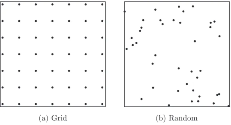
We consider regular and random patterns of facilities on a continuous plane, as shown in Figure 1. The regular and random patterns can yield analytical expressions for the distribution. The analytical expressions lead to a better understanding of fundamental characteristics of the distribution. Since actual patterns of facilities can be regarded as intermediate between regular and random, the theoretical results of these extremes will give an insight into empirical studies on actual patterns. In fact, regular and random patterns have been used in location analysis [13, 20, 23]. The regular and random patterns are assumed to continue infinitely. This assumption enables us to examine the distance without taking into account the edge effect.
(a) Grid (b) Random
Figure 1: Regular and random patterns of facilities
The distribution of the difference between the distances extends the kth nearest distance distribution, which is the distribution of the distance from a randomly selected location on a continuous plane to the kth nearest point. Analytical expressions for the kth nearest distance distribution have been obtained for regular and random point patterns. The nearest Euclidean distance was derived by Clark and Evans [4] for the random pattern, Persson [24] for the square lattice, and Holgate [9] for the triangular lattice. The kth nearest Euclidean distance was derived by Thompson [28] and Dacey [5] for the random pattern, Koshizuka [10] for k = 1, 2, 3 for the square lattice, and Miyagawa [18] for k = 1, 2, . . . , 7 for the square, triangular, and hexagonal lattices. The kth nearest rectilinear distance has also been obtained. The nearest rectilinear distance was derived by Larson and Odoni [13] for the random pattern. The kth nearest rectilinear distance was derived by Miyagawa [17] for the random pattern, and for k = 1, 2, . . . , 8 for the square and diamond lattices.
The remainder of this paper is organized as follows. The next section derives the distri-bution of the difference between the Euclidean distances to the first and the second nearest facilities. Section 3 derives the distribution of the difference between the rectilinear dis-tances. Section 4 examines the distribution of the difference between the road network distances. The final section presents concluding remarks.
2. Euclidean Distance
Let R1 and R2 be the Euclidean distances from a randomly selected location in a study region to the first and the second nearest facilities, respectively. Let V = R2 − R1 be the difference between the distances. The contour of V is given by a hyperbola, the foci of which are at facilities, as depicted in Figure 2, where points represent facilities and {p, q} represents the region where the first and the second nearest facilities are p and q. Note that
order-2 Voronoi polygon [21]. Recall that a hyperbola is defined as the locus of points such that the difference between the distances to two fixed points (foci) remains constant. In this section, we derive the distribution of the difference between the Euclidean distances V for the grid and random patterns of facilities.
1
{1,2}
{1,3}
{2,3}
2 3
Figure 2: Contour of the difference between the Euclidean distances 2.1. Grid pattern
Suppose that facilities are regularly distributed on a square grid with spacing a. The density of facilities, that is, the number of facilities per unit area is then expressed as ρ = 1/a2. Let F (v) be the cumulative distribution function of V . F (v), which is the probability that
V ≤ v, is given by
F (v) = S(v)
S , (2.1)
where S and S(v) are the area of the study region and the area of the region such that
V ≤ v in the study region, respectively. Since we assume that the grid pattern continues
infinitely, the study region can be confined to the region where two facilities are the first and the second nearest, which is the square centered at the midpoint of the facilities with side length a/√2, as shown in Figure 3. The area of the study region is S = a2/2. Set the
origin of the coordinate system O at the midpoint of the facilities. The difference between the distances from a location (x, y) to the facilities (−a/2, 0), (a/2, 0) is then
V = √( x− a 2 )2 + y2−√(x + a 2 )2 + y2 . (2.2)
The locus such that V = v is the hyperbola 4x2
v2 − 4y2
a2− v2 = 1, (2.3)
where 0 < v < a. S(v) is the area of the region between two branches of the hyperbola in the square, as shown by the light gray region in Figure 3. Then we have
S(v) = 2α(a− α) − 2 √ a2− v2 v ∫ α v/2 √ 4x2− v2 dx, (2.4)
where
α = √
2v(a2− v2)− av2
2(a2− 2v2) . (2.5)
Substituting S and S(v) into Equation (2.1) yields F (v), and differentiating F (v) with respect to v yields the probability density function of V as
f (v) = dF (v)
dv . (2.6)
f (v) for the grid pattern is shown in Figure 4(a), where the density of facilities is ρ =
1, 2, 3. It can be seen that the difference between the distances decreases with the density of facilities.
a
O
x
y
α
Figure 3: Region such that V ≤ v
(a) Grid (b) Random
1 2 3 4 0 0.2 0.4 0.6 0.8 1.0 f(v) v ρ=3 ρ=2 ρ=1 1 2 3 4 0 0.2 0.4 0.6 0.8 1.0 f(v) v ρ=3 ρ=2 ρ=1
Figure 4: Distribution of the difference between the Euclidean distances
2.2. Random pattern
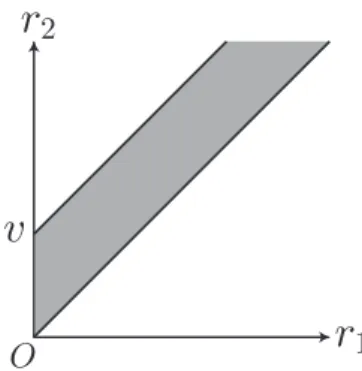
Suppose that facilities are uniformly and randomly distributed. The cumulative distribution function F (v) is obtained from the joint distribution of R1 and R2. Let f (r1, r2) be the joint probability density function of R1 and R2. f (r1, r2) for the random pattern was derived by Miyagawa [20] as
where ρ is the density of facilities. Integrating f (r1, r2) in the region such that V ≤ v on the r1–r2 plane, as shown in Figure 5, we have
F (v) = ∫∫ r2−r1≤v f (r1, r2) dr1dr2 = ∫ ∞ 0 ∫ r1+v r1 f (r1, r2) dr2dr1, (2.8) where r2 ≥ r1. Differentiating F (v) with respect to v yields
f (v) =√ρπerfc (√ρπv) , (2.9)
where erfc(·) is the following complementary error function erfc(x) = √2
π
∫ ∞
x
exp(−t2)dt. (2.10)
f (v) for the random pattern is shown in Figure 4(b). f (v) for small v for the random pattern
is greater than that for the grid pattern.
r
1r
2
O
v
Figure 5: Region such that V ≤ v on the r1–r2 plane
3. Rectilinear Distance
Although the Euclidean distance is a good approximation for the actual travel distance, the rectilinear distance is more suitable for cities with a grid road network [3, 8, 15]. In fact, the rectilinear distance has frequently been used in facility location models [1, 7, 22]. The rectilinear distance between two points (x1, y1) and (x2, y2) is defined as |x1− x2| + |y1− y2|. Let R1 and R2 be the rectilinear distances from a randomly selected location in a study region to the first and the second nearest facilities, respectively. Let V = R2 − R1 be the difference between the distances. The contour of V is given by a rectilinear hyperbola [11], as depicted in Figure 6. In this section, we derive the distribution of the difference between the rectilinear distances V for the grid and random patterns of facilities.
3.1. Grid pattern
F (v) can be obtained by the same way as the Euclidean distance case, except for replacing a
hyperbola with a rectilinear hyperbola. S(v) is the area of the region between two branches of the rectilinear hyperbola in the square, as shown by the light gray region in Figure 7, where the rectilinear hyperbola reduces to two lines. Then we have
S(v) = v
1
{1,2}
{1,3}
{2,3}
2 3
Figure 6: Contour of the difference between the rectilinear distances where 0 < v < a. Substituting S(v) into Equation (2.1) yields
F (v) = v
a2(2a− v). (3.2)
Differentiating F (v) with respect to v yields
f (v) = 2√ρ− 2ρv. (3.3)
f (v) for the grid pattern is shown in Figure 8(a). The difference between the rectilinear
dis-tances tends to be greater than that between the Euclidean disdis-tances, though the maximum is the same for the two distances (see Figure 4(a)).
a
Figure 7: Region such that V ≤ v
3.2. Random pattern
F (v) is similarly obtained from the joint distribution of R1 and R2. f (r1, r2) for the random pattern was derived by Miyagawa [20] as
f (r1, r2) = 16ρ2r1r2exp(−2ρr22). (3.4) Substituting f (r1, r2) into Equation (2.8) yields F (v), and differentiating F (v) with respect to v yields
f (v) =√2ρπerfc(√2ρv )
(a) Grid (b) Random 1 2 3 4 0 0.2 0.4 0.6 0.8 1.0 f(v) v ρ=3 ρ=2 ρ=1 1 2 3 4 0 0.2 0.4 0.6 0.8 1.0 f(v) v ρ=3 ρ=2 ρ=1
Figure 8: Distribution of the difference between the rectilinear distances
4. Road Network Distance
In this section, we evaluate the reliability of actual facility location using the distribution of the difference between the distances to the first and the second nearest facilities. As an example, we consider 32 hospitals and the road network of Setagaya, Japan, as shown in Figure 9, where open circles represent hospitals.
2 km 0
Figure 9: Hospitals and road network of Setagaya
Figure 10 shows the normalized histogram of the difference between the road network distances from all nodes to the first and the second nearest hospitals. The solid and dotted curves are the distributions of the difference between the Euclidean and rectilinear distances for the grid and random patterns with the same density of facilities. Table 1 summarizes the average and the maximum of the difference. Although the average distance for the actual pattern is smaller than that for the grid pattern, the maximum distance is greater than that for the grid pattern. This means that some customers are required to travel a long
Table 1: Average and maximum of the difference
Euclidean distance Rectilinear distance
Hospital Grid Random Grid Random
Average 0.41 0.43 0.34 0.45 0.42
Maximum 2.11 1.35 ∞ 1.35 ∞
distance when the nearest facility is closed. Thus, relocating some hospitals would reduce the difference between the distances.
0 0.5 1.0 1.5 2.0 2.5 0.5 1.0 1.5 2.0 f(v) v [km] Euc/Grid Euc/Random Rec/Grid Rec/Random
Figure 10: Distribution of the difference between the road network distances
5. Conclusion
This paper has derived the distribution of the difference between the distances to the first and the second nearest facilities. The analytical expressions for the distribution for regular and random patterns will supplement further facility location models with closing of facilities as follows. First, they give an estimate for the service level of actual facility patterns. By comparing the distributions, we can evaluate the reliability of actual patterns. Second, they demonstrate how the density of facilities affects the difference between the distances. This relationship helps planners to estimate the number of facilities required to achieve a certain level of service. The estimated number of facilities can be used as an input in location models. Note that finding the relationship between the number of facilities and the difference between the distances by using network location models requires computations for each number of facilities. Finally, they provide all the information about the difference between the distances. The average and the maximum of the difference are obtained from the distribution. The average of the difference can be used as a criterion of efficiency, whereas the maximum of the difference can be used as a criterion of equity.
We assume that customers are serviced by the second nearest facility when the nearest facility is closed. This is because customers are most likely to use the second nearest facility. If many facilities are disrupted simultaneously, however, they are required to use a more distant facility. Future research should therefore consider the difference between higher
Acknowledgements
This research was supported by JSPS Grant-in-Aid for Scientific Research. I wish to thank anonymous reviewers for their helpful comments and suggestions.
References
[1] N. Aras, M. Orbay, and I.K. Altinel: Efficient heuristics for the rectilinear distance capacitated multi-facility Weber problem. Journal of the Operational Research Society, 59 (2008), 64–79.
[2] O. Berman, D. Krass, and M.B.C. Menezes: Facility reliability issues in network p-median problems: Strategic centralization and co-location effects. Operations Research, 55 (2007), 332–350.
[3] J. Brimberg, J. Walker, and R. Love: Estimation of travel distances with the weighted
ℓp norm: Some empirical results. Journal of Transport Geography, 15 (2007), 62–72.
[4] P.J. Clark and F.C. Evans: Distance to nearest neighbor as a measure of spatial relationships in populations. Ecology, 35 (1954), 85–90.
[5] M.F. Dacey: Two-dimensional random point patterns: A review and an interpretation.
Papers of the Regional Science Association, 13 (1968), 41–55.
[6] Z. Drezner: Heuristic solution methods for two location problems with unreliable facilities. Journal of the Operational Research Society, 38 (1987), 509–514.
[7] R.L. Francis, F. McGinnes, and J.A. White: Facility Layout and Location: An
Analyt-ical Approach (Prentice Hall, Upper Saddle River, 1992).
[8] D. Griffith, I. Vojnovic, and J. Messina: Distances in residential space: Implications from estimated metric functions for minimum path distances. GIScience & Remote
Sensing, 49 (2012), 1–30.
[9] P. Holgate: The distance from a random point to the nearest point of a closely packed lattice. Biometrika, 52 (1965), 261–263.
[10] T. Koshizuka: On the relation between the density of urban facilities and the distance to the nearest facility from a point in a given area. Journal of the City Planning
Institute of Japan, 20 (1985), 85–90 (in Japanese).
[11] E.F. Krause: Taxicab Geometry: An Adventure in Non-Euclidean Geometry (Dover, New York, 1987).
[12] R.C. Larson: A hypercube queuing model for facility location and redistricting in urban emergency services. Computers & Operations Research, 1 (1974), 67–95.
[13] R.C. Larson and A.R. Odoni.: Urban Operations Research (Prentice-Hall, Englewood Cliffs, 1981).
[14] T.L. Lei and R.L. Church: Constructs for multilevel closest assignment in location modeling. International Regional Science Review, 34 (2011), 339–367.
[15] R. Love and J. Morris: Mathematical models of road travel distances. Management
Science, 25 (1979), 130–39.
[16] V. Marianov and C. ReVelle: The queueing maximal availability location problem: A model for the siting of emergency vehicles. European Journal of Operational Research, 93 (1996), 110–120.
[17] M. Miyagawa: Analysis of facility location using ordered rectilinear distance in regular point patterns. FORMA, 23 (2008), 89–95.
[18] M. Miyagawa: Order distance in regular point patterns. Geographical Analysis, 41 (2009), 252–262.
[19] M. Miyagawa: Rectilinear distance in rotated regular point patterns. FORMA, 24 (2009), 111–116.
[20] M. Miyagawa: Joint distribution of distances to the first and the second nearest facilities. Journal of Geographical Systems, 14 (2012), 209–222.
[21] A. Okabe, B. Boots, K. Sugihara, and S.N. Chiu: Spatial Tessellations: Concepts and
Applications of Voronoi Diagrams (John Wiley & Sons, Chichester, 2000).
[22] M.E. O’Kelly: Rectilinear minimax hub location problems. Journal of Geographical
Systems, 11 (2009), 227–241.
[23] M.E. O’Kelly and A.T. Murray: A lattice covering model for evaluating existing service facilities. Papers in Regional Science, 83 (2004), 565–580.
[24] O. Persson: Distance methods: The use of distance measurements in the estimation of seedling density and open space frequency. Studia Forestalia Suecica, 15 (1964), 1–68. [25] H. Pirkul: The uncapacitated facility location problem with primary and secondary
facility requirements. IIE Transactions, 21 (1989), 337–348.
[26] L.V. Snyder and M.S. Daskin: Reliability models for facility location: The expected failure cost case. Transportation Science, 39 (2005), 400–416.
[27] P. Sorensen and R. Church: Integrating expected coverage and local reliability for emergency medical services location problems. Socio-Economic Planning Sciences, 44 (2010), 8–18.
[28] H.R. Thompson: Distribution of distance to nth neighbour in a population of randomly distributed individuals. Ecology, 37 (1956), 391–394.
[29] J.R. Weaver and R.L. Church: A median location model with nonclosest facility service.
Transportation Science, 19 (1985), 58–74.
Masashi Miyagawa
Department of Regional Social Management University of Yamanashi
4-4-37 Takeda, Kofu
Yamanashi 400-8510, Japan