Vol. 61, No. 1, January 2018, pp. 151–162
CHARACTERIZING DELAUNAY GRAPHS VIA FIXED POINT THEOREM: A SIMPLE PROOF
Tomomi Matsui Yuichiro Miyamoto
Tokyo Institute of Technology Sophia University
(Received October 29, 2016; Revised November 1, 2017)
Abstract This paper discusses the problem of determining whether a given plane graph is a Delaunay graph, i.e., whether it is topologically equivalent to a Delaunay triangulation. There exist theorems which characterize Delaunay graphs and yield polynomial time algorithms for the problem only by solving some linear inequality systems. A polynomial time algorithm proposed by Hodgson, Rivin and Smith solves a linear inequality system given by Rivin, which is based on sophisticated arguments about hyperbolic geometry. Independently, Hiroshima, Miyamoto and Sugihara gave another linear inequality system and a polynomial time algorithm. Although their discussion is based on primitive arguments on Euclidean geometry, their proofs are long and intricate, unfortunately. In this paper, we give a simple proof of the theorem shown by Hiroshima et al. by employing the fixed point theorem.
Keywords: Graph theory, Delaunay graph, fixed point theorem, linear programming
1. Introduction
The two-dimensional Delaunay triangulation and its dual, the Voronoi diagram, are fun-damental concepts in computational geometry, and have many practical applications such as interpolation and mesh generation [1, 4, 9]. It is also important to recognize Delaunay triangulations. The recognition problem can be divided into two types: geometric and combinatorial. The geometric problem is to judge whether a given drawing is a Delaunay triangulation. The combinatorial problem, which is discussed in this paper, determines whether a given embedded graph is topologically equivalent to a Delaunay triangulation. The combinatorial problem is important not only theoretically but also practically because it is closely related to the design of a topologically consistent algorithm for constructing the Delaunay/Voronoi diagram in finite-precision arithmetic [8, 12, 13].
Hodgson, Rivin and Smith [6] constructed a strongly polynomial time algorithm for judg-ing whether a given 2-connected plane graph is topologically equivalent to a Delaunay tri-angulation. Their results are based on Rivin’s inscribability criterion [10, 11] of 3-connected planar graphs, which uses sophisticated arguments about hyperbolic geometry. We briefly review their results in Subsection 2.2.
Hiroshima et al. independently proposed a polynomial time algorithm [5], which solves a linear inequality system different from that appearing in [6]. Although their discussion is based on primitive arguments on Euclidean geometry, their proof is long and intricate. In this paper, we give a simple proof of their theorem in [5] by employing the fixed point theorem. After making preparations in Section 2, we discuss some properties of Delaunay graphs in Section 3 and describe our proof in Section 4.
2. Preliminaries
In this paper, for any finite set S, RS denotes the set of real vectors whose components are indexed by S.
2.1. Notations and definitions
First, we briefly review a notion of a Delaunay triangulation. Given a finite set of mutually distinct points P ⊆ R2, a Delaunay triangulation of P is commonly defined as a triangulation
of P satisfying the property that the circumcircle of each inner cell (triangle) contains no point of P in its interior. A Delaunay triangulation of P is also known as the planar dual of the Voronoi diagram of P . A Delaunay triangulation is called non-degenerate if and only if it satisfies the conditions that no three vertices on the outermost cell are collinear, and no four vertices lie on a common circle that circumscribes an inner cell.
Next, we give a definition of combinatorial triangulation. Let G′ = (V, E) be a given undirected graph with vertex set V and edge set E. We assume that G′ is a 2-connected plane graph (planar graph embedded in the 2-dimensional plane) without self-loops and parallel edges. The outermost cell of G′ is unbounded while the other cells, called inner cells, are bounded. We also assume that all the inner cells are bounded by exactly three edges. A vertex in V is called an outer vertex if it is on the boundary of the outermost cell, and an inner vertex otherwise. Similarly, an edge in E is called an outer edge if it is on the boundary of the outermost cell, and an inner edge otherwise. In the rest of this paper, we denote the set of outer vertices and the set of inner vertices by Vouter and Vinner,
respectively. For each inner cell, we associate a directed 3-cycle which is obtained from an undirected 3-cycle of G′forming boundary of the cell by directing the edges counterclockwise. Let C be the set of all the directed 3-cycles corresponding to all the inner cells of G′. A combinatorial triangulation is defined by a triplet (V, E, C). In the rest of this paper, we write G = (V, E, C) and concentrate our attention on the topological structure of G; we do not care about the actual positions at which the vertices are placed. If a given undirected graph G′ = (V, E) is 2-connected, we say that a combinatorial triangulation G = (V, E, C) is 2-connected. When a given combinatorial triangulation is 2-connected, we can define the set of outer (inner) edges and the set of outer (inner) vertices without any ambiguity.
In the following, we introduce some notions related to a problem for judging whether a given combinatorial triangulation is obtained from a Delaunay triangulation. Given a combinatorial triangulation G = (V, E, C), we seek an injection ψ : V → R2 satisfying that the set of points {ψ(v) ∈ R2 | v ∈ V } and the set of line segments between pairs in
{{ψ(u), ψ(v)} | {u, v} ∈ E} define a Delaunay triangulation. A map ψ satisfying the above conditions is called a Delaunay realization, if it exists. When a combinatorial triangulation G has a Delaunay realization, we say that G is a Delaunay graph. Especially, if a corresponding Delaunay triangulation is non-degenerate, then G is called a non-degenerate Delaunay graph. 2.2. Previous works
Hodgson, Rivin and Smith [6] proposed a strongly polynomial time algorithm for judging whether a given 2-connected combinatorial triangulation is a Delaunay graph or not. In this subsection, we briefly review their results in the non-degenerate case.
The stellation Gs of a given 2-connected combinatorial triangulation G = (V, E, C) is
a graph obtained by introducing an artificial vertex s and connecting it to all the outer vertices. The following theorem gives a necessary and sufficient condition that a given 2-connected combinatorial triangulation is a non-degenerate Delaunay graph.
Theorem 1 ([10] Theorem 13.1, [3] Lemma 2.2). A 2-connected combinatorial triangulation G = (V, E, C) is a non-degenerate Delaunay graph if and only if its stellation Gs is of
inscribable type, i.e., Gs has a (combinatorially equivalent) realization as the edges and
vertices of the convex hull of a non-coplanar set of points on the surface of a sphere in 3-dimensional space.
The following theorem gives Rivin’s inscribability criterion [10, 11].
Theorem 2 ([10, 11], [6] p.247, [3] Theorem 2.1). A graph is of inscribable type if and only if it is a 3-connected planar graph and weights w can be assigned to its edges such that: (a) for each edge e, 0 < w(e) < 1/2, (b) for each vertex v, the sum of the weights of all edges incident to v is equal to 1, and (c) for each non-coterminous cutset Γ, the sum of the weights of edges in Γ is greater than 1. (Here we note that a cutset is non-coterminous if its edges do not have a common endpoint.)
The above theorem says that we can judge whether a given 2-connected combinatorial triangulation is a non-degenerate Delaunay graph or not by checking the feasibility of the linear inequality system defined in Theorem 2. Although the number of inequalities in the linear inequality system grows exponentially in |V | (in the worst case), we can check the feasibility in strongly polynomial time (with respect to |V |) by employing the ellipsoid method (see [6] Theorem 3).
3. Characterizing Delaunay Graphs
In this section, we briefly review a set of conditions, proposed in [5], which characterizes (non-degenerate) Delaunay graphs. Given a combinatorial triangulation G = (V, E, C), we denote the elements of C by c0, c1, . . . , c|C|−1. For each (counterclockwise) directed cycle
ci ∈ C, we introduce three variables x3i+1, x3i+2, x3i+3 assigned to the three vertices in ci.
In the rest of this paper, we interpret these variables as inner angles in degrees at the corresponding corners of a triangle defined by cycle ci. We call these variables angle
vari-ables. Let vα, vβ, vγ be the three vertices of ci corresponding to the three angle variables
x3i+1, x3i+2, x3i+3, respectively. We say that x3i+1, x3i+2, x3i+3 are facing variables of
undi-rected edges {vβ, vγ}, {vγ, vα}, {vα, vβ} ∈ E, respectively. There are 3|C| angle variables
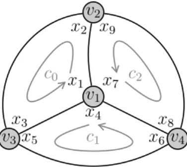
and we denotes the index set of angle variables by J := {1, 2, . . . , 3|C|}. For example, a combinatorial triangulation shown in Figure 1 has nine angle variables x1, x2, . . . , x9.
v1 x1 x4 x7 v2 x2 x9 v3 x3 x5 x6 v4 x8 c0 c1 c2
Figure 1: A combinatorial triangulation and its angle variables.
If a given combinatorial triangulation G = (V, E, C) is a Delaunay graph, there exists a vector of angle variables x ∈ RJ obtained by a Delaunay realization, which satisfies the following conditions.
C1 For each cycle in C, the sum of the associated three angle variables is equal to 180. C2 For each inner vertex, the sum of all the associated angle variables is equal to 360.
C3 For each outer vertex, the sum of all the associated angle variables is at most 180. C4 For each inner edge, the sum of the associated pair of the facing angle variables is at
most 180.
C5 Each angle variable is positive.
For example, if we consider the combinatorial triangulation in Figure 1, the above con-ditions give the following linear inequality system;
(C1) defined by c0 : x1+ x2 + x3 = 180, (C1) defined by c1 : x4+ x5 + x6 = 180, (C1) defined by c2 : x7+ x8 + x9 = 180, (C2) defined by v1 : x1+ x4 + x7 = 360, (C3) defined by v2 : x2+ x9 ≤ 180, (C3) defined by v3 : x3+ x5 ≤ 180, (C3) defined by v4 : x6+ x8 ≤ 180, (C4) defined by {v1, v2} : x3+ x8 ≤ 180, (C4) defined by {v1, v3} : x2+ x6 ≤ 180, (C4) defined by {v1, v4} : x5+ x9 ≤ 180, (C5) : x1, x2, . . . , x9 > 0.
Figure 2 gives an example of a Delaunay realization of the combinatorial triangulation in Figure 1. 30 30 30 30 30 30 120 120 120v1 v2 v3 v4
Figure 2: Realized Delaunay triangulation.
Unfortunately, the values of the angle variables satisfying all the conditions C1–C5 do not necessarily correspond to a Delaunay triangulation. For example, the combinatorial triangulation in Figure 1 has a vector of angle variables defined by
x1 = x4 = x7 = 120, x2 = x5 = x8 = 32, x3 = x6 = x9 = 28,
which satisfies C1–C5, but it does not correspond to any triangulations. If we try to draw the diagram using these angle values, we come across an inconsistency as shown in Figure 3. In order to avoid such inconsistency we need still other conditions described below.
Let c ∈ C be an inner cell with three vertices vα, vβ, vγ, and xi, xj, xk be three
angle variables corresponding to the three vertices, respectively. We say that xj is
cc-facing (meaning “cc-facing counterclockwise”) around vα and xk is c-facing (meaning “facing
clockwise”) around vα. In Figure 4, for example, x2, x5, x8 are cc-facing around v1 while
32 32 28 32 28 28 120 120 120v1 v2? v3 v4
Figure 3: Angle variables satisfying C1–C5.
v1 x1 x4 x7 v2 x2 x9 v3 x3 x5 x6 v4 x8
Figure 4: Variables x3, x6, x9 are c-facing and x2, x5, x8 are cc-facing around v1.
For any inner vertex v ∈ Vinner, let XvCC ⊆ J be indices of cc-facing angle variables around v, and XC
v ⊆ J be indices of c-facing angle variables around v. Furthermore, we
introduce a function Fv(x) := ∏ j∈XCC v sin xj ∏ j∈XC v sin xj , (3.1)
where x ∈ RJ is a vector of angle variables (in degrees). We only consider angle variables satisfying 0 < xj < 180 (∀j ∈ J), and hence we get 0 < Fv(x) <∞.
Now we describe a necessary and sufficient condition that a combinatorial triangulation becomes a Delaunay graph.
Theorem 3 ([5]). A 2-connected combinatorial triangulation G = (V, E, C) is a Delaunay graph (i.e., G has a Delaunay realization) if and only if there exists a vector of angle variables satisfying the set of conditions C1–C6, where
C6 Fv(x) = 1 for any inner vertex v ∈ Vinner.
It is not so difficult to prove the above theorem. For example, Hiroshima, Miyamoto and Sugihara gave a short and elementary proof of Theorem 3 in their paper [5], which gives a method to construct a Delaunay realization. If we restrict the Delaunay triangulations to non-degenerate ones, the conditions C3 and C4 are respectively changed in the following way.
C4’ For each inner edge, the sum of the associated pair of the angle values facing the edge is less than 180.
A non-degenerate version of Theorem 3 is as follows.
Theorem 4 ([5]). A 2-connected combinatorial triangulation G = (V, E, C) is a degenerate Delaunay graph (i.e., G has a Delaunay realization corresponding to a non-degenerate Delaunay triangulation) if and only if there exists a vector of angle variables satisfying the set of conditions C1, C2, C3’, C4’, C5 and C6.
Thus, we get a necessary and sufficient condition for a combinatorial triangulation to be a (non-degenerate) Delaunay graph. However, the conditions stated in Theorems 3 and 4 are not useful for the recognition of a Delaunay graph, because we do not know any finite-step algorithm for finding a vector of angle variables satisfying these conditions.
4. Main Result
Now we describe a linear inequality system shown in [5] which yields an efficient method for recognizing Delaunay graphs. (The method finds neither a Delaunay realization nor a vector of angle variables satisfying set of conditions C1–C6.) The following theorem says that when we only need to judge whether a given combinatorial triangulation is a Delaunay graph (or not), we can drop condition C6, surprisingly.
Theorem 5 ([5]). A 2-connected combinatorial triangulation G = (V, E, C) is a Delaunay graph (i.e., G has a Delaunay realization) if and only if there exists a vector of angle variables satisfying the set of conditions C1–C5.
It is obvious that if G is a Delaunay graph, there exists a vector of angle variables satisfying the set of conditions C1–C5. To show the inverse implication, we only need to prove that “if there exists a vector x ∈ RJ of angle variables satisfying C1–C5, then there
also exists a vector x′ ∈ RJ of angle variables satisfying C1–C6.” By employing Theorem 3, the existence of x′ ∈ RJ satisfying C1–C6 implies that G is a Delaunay graph.
We can judge the satisfiability of the set of conditions C1–C5 in finite steps because the conditions C1 through C5 are linear in the variables and the method for checking their satisfiability has been established in linear programming (see [5] for detail). Especially, the obtained linear programming problem satisfies that all the non-zero coefficients are +1 or −1, and thus it is solvable in strongly polynomial time [14].
The following theorem deals with the non-degenerate case.
Theorem 6 ([5]). A 2-connected combinatorial triangulation G = (V, E, C) is a degenerate Delaunay graph (i.e., G has a Delaunay realization corresponding to a non-degenerate Delaunay triangulation) if and only if there exists a vector of angle variables satisfying the set of conditions C1, C2, C3’, C4’, C5.
We employ the fixed point theorem and give simple proofs of Theorem 5 and Theorem 6. Theorem 7 (Fixed Point Theorem [2]).
Every continuous map f : Bm → Bm defined on an m-dimensional closed ball Bm has a fixed point (a point x∈ Bm with f (x) = x).
It is well known that we can extend the above theorem to a continuous map defined on a convex compact set.
Before describing our proof, we give a sketch of an important procedure, which transforms a feasible solution of the linear inequality system defined by C1–C5. Let us recall a vector of angle variables shown in Figure 3, that satisfies conditions C1–C5, but not C6. Now we construct a (new) vector by increasing angle variables c-facing around the inner vertex v1
by α degree, and decreasing angle variables cc-facing around v1 by α degree. After this
procedure, conditions C1–C4 are preserved. When we set α = 2, the obtained vector of angle variables, shown in Figure 2, satisfies conditions C1–C6.
Now we describe the above procedure precisely. Given a non-negative vector x ≥ 0 of angle variables satisfying C1–C4, an inner vertex v and a real number α, we introduce a vector x(v, α) defined by x(v, α)j = xj+ α, j ∈ XvCC, xj − α, j ∈ XvC, xj, otherwise. (4.1)
The following lemma shows some properties of x(v, α).
Lemma 8. Let x ≥ 0 be a non-negative vector of angle variables satisfying C1–C4 and x(v, α) be a vector defined by (4.1) w.r.t. an inner vertex v∈ Vinner. For any α∈ R, vector
x(v, α) satisfies conditions C1–C4. We define
αmax=max{α ∈ R | x(v, α) ≥ 0},
αmin= min{α ∈ R | x(v, α) ≥ 0}.
If αmin < αmax, then a real valued function Fv(x(v, α)) w.r.t. α defined on an open interval
(αmin, αmax) is a continuous monotonically increasing function.
Proof. It is easy to show that x(v, α) satisfies conditions C1–C4. The continuity of Fv(x(v, α))
with respect to α is obvious. Let C(v) ⊆ C be a set of cycles including v. For each cycle c′ ∈ C(v), angle variable xCCc′ (xCc′) denotes associated cc-facing (c-facing) angle variable
around v. Condition C1, non-negativity of x, and the inequality αmin < αmax imply that
0 < xCC
c′ + xCc′ ≤ 180 (∀c′ ∈ C(v)). We transform the following differentiation and obtain
that d log Fv(x(v, α)) dα = ∑ j∈XCC v d log sin(xj + α) dα − ∑ j∈XC v d log sin(xj − α) dα = ∑ j∈XCC v cos(xj+ α) sin(xj+ α) + ∑ j∈XC v cos(xj− α) sin(xj− α) = ∑ c′∈C(v) ( cos(xCCc′ + α) sin(xCC c′ + α) +cos(x C c′ − α) sin(xC c′ − α) ) = ∑ c′∈C(v) sin(xCC c′ + xCc′) sin(xCC c′ + α) sin(xCc′ − α) > 0,
where the last inequality is derived from the facts that (1) ∀α ∈ (αmin, αmax), ∀c′ ∈ C(v),
sin(xCC
c′ + α) sin(xCc′ − α) > 0 (2) ∀c′ ∈ C(v), sin(xcCC′ + xCc′) ≥ 0, and (3) ∃c′ ∈ C(v),
sin(xCCc′ + xCc′) > 0 (obtained from C2). Thus, both log Fv(x(v, α)) and Fv(x(v, α)) are
monotonically increasing in α.
In our proof of Theorem 5, we adopt the above procedure around all inner vertices simultaneously.
Proof. (Proof of Theorem 5.) From Theorem 3, we only need to show that once we obtain a vector of angle variables satisfying C1–C5, there exists a vector of angle variables satisfying C1–C6.
Let b ∈ RJ be a vector of angle variables satisfying conditions C1–C5. We define a
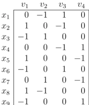
matrix M whose rows are indexed by J ={1, 2, . . . , 3|C|} (the index set of angle variables), columns are indexed by the vertex set V , and each entry miv is defined as follows:
miv=
1, if angle variable xi is cc-facing around v,
−1, if angle variable xi is c-facing around v,
0, otherwise.
Figure 5 shows a matrix M corresponding to Figure 1.
v1 v2 v3 v4 x1 0 −1 1 0 x2 1 0 −1 0 x3 −1 1 0 0 x4 0 0 −1 1 x5 1 0 0 −1 x6 −1 0 1 0 x7 0 1 0 −1 x8 1 −1 0 0 x9 −1 0 0 1
Figure 5: A matrix M corresponding to Figure 1.
Let fM be a column submatrix of M corresponding to inner vertices Vinner. It is easy to
see that the vector of angle variables fM y +b is obtained from b by decreasing angle variables c-facing around the inner vertex v by yv, and increase angle variables cc-facing around v by
yv, for each inner vertex v ∈ Vinner. The definition of fM directly implies that for any vector
y∈ RVinner
, a vector of angle variables fM y + b also satisfies conditions C1–C4. We introduce a closed subset Ω ⊆ RVinner defined by
Ω := {
y∈ RVinner fM y + b≥ 0 }
.
Here, we briefly show the boundedness of Ω by contradiction. Motzkin [7] showed that the set of all the solutions of a given linear inequality system can be written as the Minkowski sum of a (bounded) polytope and a cone. From Motzkin’s theorem, the unboundedness of Ω implies the existence of a ray vector y′ ∈ RVinner of Ω satisfying fM y′ ≥ 0. We define
V± = {v ∈ Vinner | yv′ ̸= 0}. Since V± ⊆ Vinner, there exists an inner edge connecting a vertex v ∈ V± and a vertex in V \ V±, and thus vertex v has a pair of angle variables x and x′ which are c-facing and cc-facing around v, respectively. If yv′ is positive (negative), then a component of fM y′ indexed by x (x′) is negative, which contradicts with the assumption
f
M y′ ≥ 0. From the above, Ω is a compact convex set.
For any pair (y, v)∈ Ω × Vinner, we define following two values: αmax(y, v) := max{α ∈ R | y + αev ∈ Ω},
αmin(y, v) := min{α ∈ R | y + αev ∈ Ω},
where ev ∈ {0, 1}V
inner
is a unit vector whose entry is equal to 1 if and only if the corre-sponding index is equal to v. (Here we note that both the maximum and the minimum
always exist, because Ω is a bounded closed set and is nonempty; clearly b ∈ Ω.) Since y ∈ Ω, inequalities αmin(y, v) ≤ 0 ≤ αmax(y, v) hold. When αmin(y, v) < αmax(y, v), we
have that lim α→αmax(y,v) Fv(y + αev) = +∞, (4.2) lim α→αmin(y,v) Fv(y + αev) = +0, (4.3)
and thus Lemma 8 and the intermediate value theorem imply that there exists a unique value α∗ in the open interval (αmin(y, v), αmax(y, v)) satisfying equality Fv(y + α∗ev) = 1.
Now we introduce a map fv : Ω→ Ω for each v ∈ Vinner defined by
fv(y) =
{
y, if αmin(y, v) = αmax(y, v) = 0,
y + α∗ev, if αmin(y, v) < αmax(y, v),
where α∗ is a unique value satisfying Fv(y + α∗ev) = 1. It is obvious that for each inner
vertex v, the corresponding map fv is continuous.
Lastly, we define a map f : Ω → Ω as: f (y) := 1
|Vinner|
∑
v∈Vinner
fv(y),
where f (y) is the gravity center of vectors {fv(y) | v ∈ Vinner}. Since fv is continuous for
each inner vertex v, f is also continuous.
Now we apply the fixed point theorem to the continuous map f and obtain a result that there exists a fixed point y∗ ∈ Ω, i.e., y∗ satisfies f (y∗) = y∗.
Every fixed point y∗ satisfies that ∀v ∈ Vinner,
αmin(y∗, v) = αmax(y∗, v) or Fv(y∗) = 1.
(4.4) Otherwise, there exists at least one inner vertex v′ satisfying αmin(y∗, v′) < αmax(y∗, v′)
and Fv′(y∗) ̸= 1. Then v′ also satisfies fv′(y∗) ̸= y∗, which implies f (y∗) ̸= y∗. It is a
contradiction.
It is obvious that every fixed point y∗ ∈ Ω satisfies C1–C4. Next we discuss condition C5, i.e., we show that fM y∗+ b > 0 for any fixed point y∗.
If a vertex v satisfies αmin(y∗, v) = αmax(y∗, v), then αmin(y∗, v)≤ 0 ≤ αmax(y∗, v)
im-plies αmin(y∗, v) = αmax(y∗, v) = 0. When a vertex v satisfies αmin(y∗, v) < αmax(y∗, v),
property (4.4) gives the equality Fv(y∗) = 1. In this case, (4.2) and (4.3) imply 0 <
αmax(y∗, v) and αmin(y∗, v) < 0, respectively. From the above discussion, we have shown
that for any v∈ Vinner,
αmin(y∗, v) = 0 if and only if αmax(y∗, v) = 0. (4.5)
Let x∗ = fM y∗ + b. If an inner vertex v has a cc-facing angle variable xj satisfying
x∗j = 0, then αmin(y∗, v) = 0 and thus αmax(y∗, v) = 0, which implies that v also has a
c-facing angle variable xj′ satisfying x∗j′ = 0. Similarly, when an inner vertex v has a c-facing
angle variable xj satisfying x∗j = 0, then αmax(y∗, v) = 0 and thus αmin(y∗, v) = 0, which
Let us consider a directed graph H whose incident matrix is M⊤: i.e., a directed graph obtained from G by substituting a pair of parallel arcs with opposite direction for each inner edge in E and directing outer edges in E appropriately (see Figure 6). Digraph H has vertex set V and arc set J , which is an index set of angle variables. Each angle variable xj corresponds to an arc in H from u to v where xj is a c-facing variable around u and
cc-facing variable around v.
v1 v2 v3 v4 x1 x2 x3 x4 x5 x6 x7 x8 x9
Figure 6: A directed graph H = (V, J ) corresponding to Figure 1.
If an arc a of H satisfies that the corresponding angle variable, denoted by xa, satisfies
x∗a = 0, we say that a is a critical arc. In the directed graph, each inner vertex v satisfies that v has an incoming critical arc if and only if v has an outgoing critical arc. It is because, property (4.5) implies that v has a cc-facing angle variable xj satisfying x∗j = 0 if and only if
v has c-facing angle variable xj′ satisfying x∗j′ = 0, and xj and xj′ correspond to an incoming
critical arc and an outgoing critical arc of v, respectively.
Now we show x∗ > 0. Assume on the contrary that there exists an angle variable xj
satisfying x∗j = 0. Then, there exists a critical arc in H. Let A0 be the set of all the critical
arcs. From the above discussion, a digraph defined by (V, A0) has either (Case 1) “a directed
elementary path Γ1 connecting a pair of outer vertices and passing only inner vertices” or
(Case 2) “a directed elementary cycle Γ2 consisting of inner vertices.” (Here we note that a
path is called elementary if no vertices appear more than once in it. An elementary cycle is a closed walk with no repeated vertices or edges aside from the necessary repetition of the start and end vertex.)
Case 1. Let χ1 ∈ {0, 1}J be a characteristic vector of the set of arcs in path Γ1. Since Γ1
consists of critical edges, χ⊤1x∗ = 0 hold. Every inner vertex v is not a terminal vertex of Γ1,
and thus v has an incoming arc in Γ1 if and only if v has an outgoing arc in Γ1. Accordingly,
the equality χ⊤1M = 0 hold. Thus we have thatf
0 = χ⊤1x∗ = χ⊤1( fM y∗+ b) = χ⊤1M yf ∗+ χ⊤1b = χ⊤1b > 0. Contradiction.
Case 2. Let χ2 ∈ {0, 1}J be a characteristic vector of the set of arcs in cycle Γ2. Since Γ2
consists of inner vertices and critical edges, both χ⊤2M = 0 and χf ⊤2x∗ = 0 hold. Thus we have that
0 = χ⊤2x∗ = χ⊤2( fM y∗+ b) = χ⊤2M yf ∗+ χ⊤2b = χ⊤2b > 0. Contradiction.
Lastly, we show that every fixed point y∗satisfies C6. Since every fixed point y∗ satisfies C5, i.e., x∗ = fM y∗ + b > 0, every inner vertex v satisfies αmin(y∗, v) < 0 < αmax(y∗, v).
From property (4.4), equality Fv(y∗) = 1 holds at every inner vertex v. As a consequence,
condition C6 is satisfied.
A proof of Theorem 6 is almost the same. Actually, we only have to replace C3 and C4 with C3’ and C4’ respectively in our proofs of Lemma 8 and Theorem 5.
Acknowledgment
We wish to express our thanks to Naoyuki Kamiyama and Mizuyo Takamatsu for fruit-ful discussions. We would like to thank Kokichi Sugihara for introducing this interesting problem. We also thank anonymous reviewers.
References
[1] F. Aurenhammer: Voronoi diagrams - a survey of a fundamental geometric data struc-ture. ACM Computing Surveys, 23 (1991), 345–405.
[2] L.E. Brouwer: Uber Abbilidungen von Mannigfaltigkeiten. Mathematische Annalen,¨ 71 (1912), 97–115.
[3] M.B. Dillencourt and W.D. Smith: Graph-theoretical conditions for inscribability and Delaunay realizability. Discrete Mathematics. 161 (1996), 63-77.
[4] H. Edelsbrunner: Algorithms in Combinatorial Geometry (Springer, Heidelberg, 1987). [5] T. Hiroshima, Y. Miyamoto, and K. Sugihara: Another proof of polynomial-time rec-ognizability of Delaunay graphs. IEICE Transactions on Fundamentals of Electronics, Communications and Computer Sciences, E83-A (2000), 627–638.
[6] C.D. Hodgson, I. Rivin, and W.D. Smith: A characterization of convex hyperbolic polyhedra and of convex polyhedra inscribed in the sphere. Bulletin of the American Mathematical Society, 27 (1992), 246–251.
[7] T.S. Motzkin: Beitr¨age zur Theorie der linearen Ungleichungen. Inaugural Dissertation Basel, Azriel, Jerusalem, 1936.
[8] Y. Oishi and K. Sugihara: Topology-oriented divide-and-conquer algorithm for Voronoi diagrams. CVGIP: Graphical Model and Image Processing, 57 (1995), 303–314.
[9] A. Okabe, B. Boots, K. Sugihara, and S.N. Chiu: Spatial Tessellations: Concepts and Applications of Voronoi Diagrams (Wiley and Sons, England, 2nd edition, 2000). [10] I. Rivin: Euclidean structures on simplicial surfaces and hyperbolic volume. Annals of
Mathematics, 139 (1994), 553–580.
[11] I. Rivin: A characterization of ideal polyhedra in hyperbolic 3-space. Annals of Math-ematics, 143 (1996), 51–70.
[12] K. Sugihara and M. Iri: Construction of the Voronoi diagram for “one million” gener-ators in single-precision arithmetic. Proceedings of the IEEE, 80 (1992), 1471–1484. [13] K. Sugihara and M. Iri: A robust topology-oriented incremental algorithm for Voronoi
diagrams. International Journal of Computational Geometry & Applications, 4 (1994), 179–228.
[14] E. Tardos: A strongly polynomial algorithm to solve combinatorial linear programs. Operations Research, 34 (1986), 250–256.
Tomomi Matsui
Department of Industrial Engineering and Economics, Graduate School of Engineering,
Tokyo Institute of Technology,
Ookayama, Meguro-ku, Tokyo 152-8550, Japan. E-mail: [email protected]