Society of Japan
Vol. 31, No. 3, September 1988
A DUAL INTERIOR PRIMAL SIMPLEX METHOD
FOR LINEAR PROGRAMMING
Akihisa Tamura Tokyo Institute of Technology
Hitoshi Takehara University of Tsukuba
Komei Fukuda Tokyo Institute of Technology Satoru Fujishige
University of Tsukuba
Masakazu KOjima Tokyo Institute of Technology
(Received October 29,1987; Revised May 2,1988)
Abstract This paper proposes a hybrid computational method (DIPS method) which works as a simplex method for solving a standard form linear program, and, simultaneously, as an interior point method for solving its dual. The DIPS method generates a sequence of primal basic feasible solutions and a sequence of dual interior feasible solutions interdependently. Along the sequences, the duality gap decreases monotonically. As a simplex method, it gives a special column selection rule satisfying an interesting geometrical property.
Key Words: Linear programming, interior point method, simplex method.
1 Introduction.
We consider the standard form linear program:
p
and its dual
D maxImIze subject to mInimize subject to Jl E X =
{:z:
~ 0I
A:z: = b} bTy YEY={yIATy~C}where A denotes an m x n matrix, b an m-dimensional column vector and c an n-dimensional column vector. Throughout the paper we impose the following assump-tions.
414 A. Tamura, H. Takehara, K. Fukuda, S. Fujishige & M. Kojima
Assumption 2. There is an :c in the primal feasible region X such that :c
>
o. Assumption 3. The dual feasible region Y has a nonempty interior, i.e., there exists y such that AT y>
c.The well-known duality theorem ensures that both of the problems P and D have optimal solutions with a common optimal value A *.
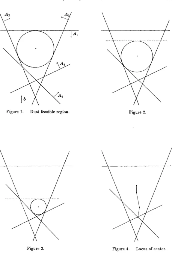
A dual-interior primal-simplex method (DIPS method), which we propose in this paper, has some interpretations. First it can be viewed as an interior point algorithm for solving the dual problem D. Suppose that the steepest descent direction -b of the objective value of the dual problem D coincides with the gravitational direction and that the vertical axis represents the objective value bT y (See Figure 1). It will be convenient for our discussion here to consider the dual feasible region Y as a vessel. We fill the vessel with the water to some level A and make a hole at the bottom of the vessel which corresponds to a minimal solution of the dual problem D with the objective value A*. Then the level A of the water goes down until the vessel is empty. For each level A of the water, we consider a maximal ball S with a center y under the water. As the level A of the water goes down, the maximal ball S shrinks with the center y moving down, and finally the center y will reach the bottom (the minimal solution of the dual problem D) when the vessel becomes empty (or the level A attains the minimal value A* of the problem D). In this process the locus of the center forms a piecewise linear curve. See Figures 2, 3 and 4. Given an initial maximal ball with a center yi and a water level Ai, the DIPS method traces the locus of the center to attain a minimal solution of the dual problem D.
The DIPS method may be regarded as a modification of the gravitationa.l method given by Murty [7] and Chang and Murty [2]. Their method is outlined as follows. If we pick up a small heavy ball and release it at some point in the interior of the vessel (the dual feasible region Y), the ball is falling and rolling down by the gravitational force and stops when it minimizes the potential energy (or equivalently its center minimizes the dual objective function). In this physical process, the center of the ball draws a piecewise linear locus with each piece of line parallel to either the gravitational direction or some of the facets of Y. Their method traces this piecewise linear locus. If the ball is sufficiently small, we have an approximate minimal solution. Otherwise, we replace the ball by a smaller one and release it at some interior point under the end of the locus to repeat the same process. They have also devised an additional technique for finding an exact solution of D in a finite number of steps.
In the gravitational method, the ball maintains its size as long as it can decrease the potential energy, while the DIPS method deals with a ball which can not decrease the
Figure 1. Dual feasible region. Figure 2.
416 A. Tamura. H. Takehara. K. FIIIa*. S. Fujishige & M. Kojima
potential energy unless it gets smaller; thus the ball shrinks continuously to decrease the potential energy.
The DIPS method can also be viewed as a primal simplex method with a certain column selection rule. In Section2, it will be shown the sequence {yk
I
k = 1,2, ... } of the nodal points of the piecewise linear locus of the cent er of the maximal ball induces a sequence {:Jl"I
k = 1, 2, ... } of basic feasible solutions of the primal problem P such that eT:JlkS
eT :Jllc+l; the DIPS method generates an interior feasible solution yk of the dual problem D and a basic feasible solution :Jllc of the primal problem P interdependently. Therefore,(a) we have an upper bound bT
yI'+1
and a lower bound eT:Jlk for the unknownoptimal value A* throughout the iteration,
(b) the duality gap bT
yk+l - eT:Jlk decreases as the iteration proceeds,
(c) both of primal and dual optimal solutions are generated in at most a finite number of steps.
In Section 3, we give another interpretation to the DIPS method in terms of para-metric linear programs (see, for example, [3]). From this interpretation, we will derive an interesting geometrical property on the sequence {:Jlk
I
k = 1,2, ... } of basic feasible solutions of P generated by the DIPS method.A drawback of the DIPS method is that we need in advance a maximal baY with a certain additional property in the dual feasible region to start the itera.tion. We can utilize the gravitational method referred above to prepare such a maximal ball:, we can switch from the gravitational method to the DIPS method when the ball with a fixed. size used in the former minimizes the potential energy and stops f1WOng. In Section 4, the DIPS method is modified so that it can start from any pair of a dual interior feasible solution and a primal basic feasible solution. This modification will make it easier to incorporate the DIPS method into other interior point methods (Karmarkar [4], Kojima, Mizuno and Yoshise [5], Renegar [8], Todd and BurreH [9], etc.) developed recently.
2 Details of The DIPS Method.
In the previous section, we illustrated a hehavior of the DIPS metho,d as an interior point algorithm for solving the dual problem D. In this section, we will describe the details of the DIPS method and relate it to a simplex method for solving the primal problem P.
We begin by writing the constraints of the dual problem D as
where Ai denotes the ith column vector of A and C; the ith element of c. In the previous section, we compared the dual feasible region Y to a vessel which we filled with the water to some level A. The level A of the water corresponds to the hyperplane
and the region YeA) under the water is defined by
Here A moves from a sufficiently large positive number to the minimum value A * of the dual problem D. It is easily verified under Assumptions 1, 2 and 3 that yeA) is bounded for every A ~ A *.
For every yE Rm and r
>
0, let S(y, r) denote the ball with the center y and the radius :r, i.e., S(y, r) = {y E Rmlily - YII
S
r}. For simplicity of notation, we shall assume thatIIAdl
= 1 (i = 1,2, ... , n) andIIbll
= 1.We can always rescale the primal problem P and the dual problem D so that the above equalities are satisfied. Then a ball S(y, r) is included in yeA) if and only if the inequalities
A[y-c; ~ I' (i=1,2, ... ,n) and
A - bTy ~ r
hold. For every ball S(y, r) in the dual feasible region Y, let U(y, r) be the collection of indices of the hyperplanes {y E Rm
I
Af
y - C; =o}
of Y which support the ball, l.e.,(2.2)
U(y,r) = {iE{l, ... ,n}I
A[y-c;=r}.Since yeA) is bounded for any A ~ A*, there exists a ball which is included in yeA) and has the maximum radius. We call such a ball a maximal ball at level A or A-maximal ball. We say that a A-maximal ball S(y, r) is proper if it satisfies the following two conditions:
Condition 1.
y
minimizes the objective function of the dual problem D among the centers of A-maximal balls;Condition 2. U(y,r) is maximal among all U(y,r)'s such that S(y,r) is a A-maximal ball satisfying Condition 1.
The following theorem is essentially due to Murty [7]. We include a proof for complete-ness.
418 A. Tamura, H. Takehara, K. Fukuda, S. Fujishige & M. Kojima
Theorem 1. (Theorem 1 in (7] and Theorem 5 in (2]) For every proper maximal ball S(y, r) at level A, there exists a feasible basis B of the primal problem P such that B ~ U(y, r).
Proof. For simplicity of notation, let U = U(y, r). Let E be the subspace spanned by the column vectors Ai (i E U), and El. be its orthogonal complement {y E Rm
I
(Au )T Y = o} where Au denotes the m xI
UI
matrix consisting of all the column vectors Ai with i E U. If the orthogonal projectionb
of b onto the subspace El. were not zero, we could move the center of the ball S(y, r) slightly in the direction-b
so that the ball would remain in Y(A) and that the value of the dual objective function bTy
at the cent er would decrease. This would contradict Condition 1. Henceb
= 0 or b is contained in the subspace E.Now we shall show that rank(Au)
=
m. Assume on the contrary that rank(Au)<
m. By Assumption 1, we know that rank(A) = m. Hence we can find a column vector A j , jfI
U, of the matrix A for which AjfI
E; hence the orthogonal projection v of Aj onto El. is nonzero. Therefore, if we move the cent er of the ball in the direction -v so long as the ball remains in the bounded region Y()'), the number of the boundary hyperplanes {y E RmI
AT
y-
Ct = r} of Y which support the ball increases by at least one. It should be also noted that any movement of the center of the ball S(y, r) in the direction -v never changes the dual objective value at the eenter since bEE. This contradicts Condition 2, the maximality of the index set U. Thus we have shown that rank(Au) = m.By the Condition 1 imposed on the proper maximal ball S(y, r) and the definition (2.2) of the index set U, there is no direction v E Rm such that
and
for all i E U.
Hence, by applying the well-known Farkas' Lemma, we see that there is a feasible solution :c E X of the primal problem P such that Xj = 0 (j
fI
U). Since rank(Au) = m, wecan choose a basic feasible solution ai from the set of such feasible solutions. Finally, letting B be the primal feasible basis associated with ai, we obtain B ~ U. 0
We call a ball S(fJ, r) ~ Y such that U(y, r) contains a feasible basis B of the primal problem P a basic ball in Y. By Theorem 1, every proper maximal ball is a basic ball. Conversely, we can prove similarly that if S(
y,
r) is a basic ball and we set A to be r+ b
T11
then S(y, r) is a proper A-maximal ball.pair of subproblems:
P
u Du maXlmlze subject to mlnlmlze subject to (CU)T:c Au:c = b, :c2:
o.where U denotes the index set U(y, r). By the definition of a basic ball, we know that the problem Pu has at least one feasible basis and that
y
is a feasible solution of the problem Du. Hence, by the duality theorem, the problem Pu has an optimal basis. Theorem 2. Let S(y, r) be a basic ball and U = U(y, r). Suppose that B is an optimal basis of the problem Pu . Let v = (A~)-lCB - y. Then- r = ATv ~ AJv for all i E B and all j E U\B.
Proof. Let,~
=
(A~)-lCB' Thenz
is an optimal solution of the dual problem Du.Assume on the contrary that B does not satisfy the condition, i.e., there exist i E B and j E U\B such that
(2.3) AT v
>
AJ v. Since i, j E U, we have (2.4) Henceo
A T i fI- ci = AT-j Y - Cj = r. ATz - ci = ATy+ATv-Ci = AJY
+ AT v -
Cj>
A:rJ y-+A:rv - c' J J (since i E B) (since z= y
+
v) (by (2.4)) (by (2.3))AJz-cj. (since z=fI+V)
Thus we obtain 0
>
AJz -
Cj. This contradicts the feasibility of the optimal solution z of the problem Du. 0For every feasible basis B of the primal problem P, let :E(B) denote the collection of all the basic balls S(y, r) with B ~ U(fI, r), and let C(B) denote the set of all the centers fI of basic balls S(y, r) with B ~ U(fI, r), i.e.,
C(B)
=
{y E RmI
S(y, r) E :E(B), r2:
o}.Theorem 3. Let B be a feasible basis of the primal problem P. If the set C(B) is nonempty, it forms a closed interval (closed convex subset) of the line
L(B) = {y E Rm
I
y = s(A~)-le
+
z for all s ER} where e =(1, ... , If E
RB and z = (A~)-lCB'420 A. Tamura. H. Takehara. K. Fukuda. S. Fujishige & M. Kojima
Proof. Let S(y, r) be a basic ball. Since A[Y - Ci
=
r for allr(A~)-1e
+
z,
i.e., y lies on the line L(B).Let S(yP, rP)
(p
= 0, 1) be basic balls in ~(B). Then (2.5)E B,
Y
=hold for all i E B. Suppose that S(yt, rt) is a ball with a center yt = (1 - t)y0
+
ty1and a radius rt
=
(1 - t) rO+
t r1 for some t E [0,1). By (2.5), it is clear thatAryt - Ci = rt for all i E B. We also see from the convexity of the dual feasible region
Y that S(yt, rt) ~ Y. Thus S(yt, rt) is a basic ball with B ~ U(yt, rt). Thus we have shown that C(B) is convex. The closedness of C(B) follows from the closedness of Y. 0
Now we are ready to explain the detail of the DIPS method. The method generates a sequence {S(yk, rh)} of basic balls, a sequence {Bh} of primal feasible bases and a sequence
{2)h}
of primal basic solutions which satisfy(2.6) (2.7) (2.8) (2.9) (2.10) (2.11) (2.12) rhH = min{r
I
S(y, r) E ~(Bh)}, B" ~ U(y", r"), B" ~ U(flIc+1, rIcH),ATv::; AJv for all iEBh and all jEU(y",rh)\B", bTy lc+1
<
bTy" andr lor every k =" ... , 1 2 were h v = (AT Bk )-1 CBk - Y . -le
The iteration starts with an initial basic ball S(y1, r1), which is assumed to be available in advance. Let U = U(y1, r1), and solve the subproblem Pu for this U to obtain an optimal solution 2)1 and the corresponding optimal basis B1. Let
v = (A~d-1CBl - y1. Then, by Theorem 2, we have
Now we suppose that we have obtained a basic ball S(yh, rh) and a primal feasible
Bh satisfying (2.8) and (2.10), and show how to generate a new basic ball S(
yh+l, r"+1),
a primal basic feasible solution 2)1c+1 and a primal basis Blc+1 at the kth iteration. Let Zh = (A~k)-1cBL Then v can be rewritten as v = zh -
f/.
For each t E [0,1]' we consider a ball with the cent er y"(t) = y"+
tv and the radiusrk(t)
=
aTf/'(t) - C=
(1 - t)rk where a =: Ai and C=
Ci for some i E Bk. (Note that rk(t) is independent of any selection of i E Bk). Then(2.13) for all t E [0,1] and all i E Bh.
For any sand t with 0::; s
<
t ::; 1 and i EB",
we also have (2.14) r"(s) - r"(t)=
(t - s)r">
o.
Hence, as t increases from 0, the ball 5(yk(t), r"(t» shrinks and its center 1/(t)
moves linearly toward
z".
Specifically,(2.15) yk(1)
=
z" and r"(1)=
O.In other words, the ball 5(y"(t), r"(t» shrinks into the point Zk when t = 1.
By (2.13), we see that if the ball 5(yk(t), r"(t» lies in the dual feasible region Y for some t E [0,1] then it is a basic ball. By Theorem 3, we know that the set of such
t's forms an interval. Let
pc
be the maximum value among such t's. Then(2.16) for all t E [0, PC] and all j ~ B".
We have either [k
=
1 or [" E [0,1). Let y"+l = y"([h) and rh+1 = r"([h).First we consider the case that
pc
=
1. It follows from (2.13), (2.15) and (2.16) that yk+1=
Zh is a dual feasible solution with the objective value bT z"=
c~~Alilb.Since B" is a primal feasible basis, we obtain, by the duality theorem, that y"+l is an optimal solution of the dual problem D and Bh is an optimal basis of the primal problem P. In this case, the DIPS method stops.
Now we consider the case that
pc
E [0,1). By the definition of [", we can find an index e ~ B" such thatA;y"([") - Ce = rk([k),
(2.17) A;yk(l"+e)-ce
<
r"(l"+e) for any e>O,S(y"+1,rk+1) ~ Y and B" U {e} ~ U(yk+1,rk+1).
That is, S(y"(t), r"(t» bumps against the eth constraint of (2.1) when t attains
i"k,
and then we have a new basic ball S(yk+1, rk+1) satisfying (2.9). Taking ["
+
e=
1 in (2.17), we have(2.18)
(see also (2.15». We shall show that (2.6). It follows from (2.17) and y"(t) =
fJ"
+
422 A. Tamura. H. Takehara. K. Fukuda. S. FUjishige & M. Kojima
for every sufficiently small positive €. On the other hand, by (2.14), we have
for every sufficiently small positive € and every i E B". Hence
(2.19) for every i E B".
Since B" and v satisfy (2.10), we see e ~ U(y", r"), i.e.,
A;
y"(O) - Ce>
r" = r"(O).Comparing the inequality above with (2.17), we have t"
>
0, and (2.6) follows from (2.14).To see (2.11), we evaluate the dual objective function at yk+1 : bTy lc+1 bT(y"
+
{"v)= bT(y" +t"(Zh - yh»
= bTylc
+
t"(bT(A~~)-1CBk - bTylc) = bT y"+
P'{ C~k (ABk )-1b - bT yk}.Since B" is a primal feasible basis and
y"
is a dual interior feasible solution, by the duality theorem, we see that the term in the {} of the right hand side of the last equality above is negative. Thus we obtain (2.11).We have shown that the new ball S(yIc+1, r1c+1) is a basic ball with Bh C
U(yk+l, rH1 ). In view of Theorem 3, both y" and yH1 lies on the line
Furthermore, by the construction, we see that ylc+l is an extreme point of the interval
G(Bk) of all the centers of basic balls S(y, r) E ~(Bh). Since the radius of the ball
S(y, r) changes linearly on C(B"), by (2.14), we obtain (2.7).
Now we will choose a new primal feasible basis B = B"+1 ~ U(yIc+1, rk+1) such that (2.20)
where v = (A~)-1CB - yH1. It should be noted that the old basis B == B" does not satisfy the above relation any more because of (2.19) and e E U(yHl, rlc+1). Let
B
=
Blc+l be an optimal basis of the subproblem Pu with U=
U(yHl, rHl), and ;llk+1 be the basic feasible solution of the problem P associated with the basisBIc+1. By Theorem 2, the relation (2.20) holds. Since BI< is also a feasible basis of the subproblem Pu , the inequality (2.12) follows.
iteration the radius of the cent er of primal feasible primal basic th e basic ball the basic ball basis feasible solu tion
rl
1l
Bl :cl 11
/
/
r2fi
B l _ B 2 :c l _ :c~ 21
/
/
r3fl
B 2 _ B3 :c2 _ :c 3 ~ / ' / ' / ' / ' M _M BM~BM M-I M r y :c ---+-:c M1
/
/
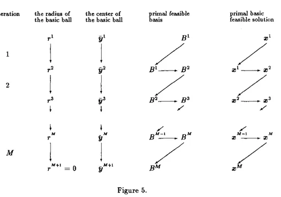
M+I =0 _M+I BM :cM r y Figure 5.Thus we have generated all the new iterates, the basic ball S(yk+l, ricH), the primal feasible basis Bk+l and the associated basic feasible solution :cIcH of the problem P,
and confirmed that all the relations (2.6) through (2.12) are satisfied. Replacing k by
(k
+
1), the DIPS method repeats the same process.The relations (2.6) and (2.7) ensure that each primal feasible basis appears in the sequence {BIc} at most once. For if BIc =: B Ic' for some distinct k and k', we would have from (2.7) that rk+l = rlc'H, which would contradicts (2.6). Therefore, we can conclude that the DIPS method terminates in a. finite number, say M, of iterations. Figure 5 illustrates the iterates of the DIPS method. Here yMH is an optimal solution of the dual problem D and :cM is an optimal solution of the primal problem P.
In each iteration, we need to compute an optimal basis Blc+l of the subproblem Pu with U
=
U(yk+l, rlc+l). As we have observed, BIc is a feasible basis of the subproblemP
u . Hence we can apply the phase 2 of the standard primal simplex method with the initial feasible basis BIc to the subproblem Pu . This may take more than one pivot iterations generally. If the nondegeneracy assumption below is satisfied, however, only one pivot iteration is required to solve the subproblem Pu .Assumption 4. (Dual Nondegeneracy Assumption). For any basic ball S(y, r), the index set U(y, r) has no more than m
+
1 elements.424 A. Tamura, H. Takehara, K. Fukuda, S. Fujishige & M. Kojima
U = BIoU{ e} for a unique index e
f/.
U(t/, rk) satisfying (2.17). Hence, the subproblem Pu with U=
U(yio+l, rio+l) has exactly two feasible basis, which are nondegenerate and adjacent with each other; the one is Bk and the other is BH1. Thus we need exactly one pivot operation to compute Bio+l from B". If, in addition, the primal nondegeneracy assumption below is satisfied, the value of the objective function of the problem Pu (hence P) increases by the pivot operation, i.e., eT :cH1>
eT;ck smcethe simplex criterion Ce - A~(A~t)-leBt is positive by the inequality (2.18).
Assumption 5. (Primal Nondegeneracy Assumption). For every feasible basis B of the primal problem P, the inequality A81b
>
0 holds.Therefore, if we restrict our attention to the sequence {:ck} of basic feasible solutions of the primal problem P, the DIPS method may be regarded as a primal simplex method with a special column selection rule using the information on basic balls in the dual feasible region. In the next section, a certain interesting property on the sequence
{Zk}
will be shown.In degenerate cases where Assumptions 4 and/or 5 are not satisfied, it may be nec-essary to incorporate some technique to avoid cycling in the simplex method for solving the subproblem Pu . For example, we can employ the smallest-subscript pivoting rule by Bland
[1].
3 An Interpretation of The DIPS Method in terms of Parametric
Program-ming.
Let
{S(l/, rh)
I
k
= 1, ... ,M
+
1} be the sequence of basic balls,{B"
I
k
= 1, ... , M} the sequence of primal feasible bases and {zkI
k = 1, ... , M} the sequence of primal basic solutions which are generated by the DIPS method. We will relate these sequences to the following primal-dual pair of parametric programsP(r) D(r) maxImIze subject to mmlmlze subject to :c
:?:
0,Here r is a scalar parameter and e denotes the vector of ones with the dimension n. Obviously, P(O) and D(O) are the same linear programs as P and D, respectively.
First we observe that each ;eh is a basic feasible solution, with the basis BI<, of the problem Per) for every r. Hence we have
x~ 3
=
0x~+1 = 0
3
for all j (j. Bh and for all j (j. BH!.
We also see that each flHI is a feasible solution of the problem D( rH!).
By
the definition of U(flHI, rHI), we haveThe three equalities above, together with the relations (2.8) and (2.9), imply the com-plementary slackness condition holds between ;eh and flHI, and between ;eH! and
flH1, respectively. Hence, ;eh and ;eHI are both optimal solutions of the primal
problem P(rlc+!) and that fllc+l is an optimal solution of the dual problem D(rk+l).
Thus we obtain
(3.1) (k=1,2, ... ).
The above discussion indicates that the DIPS method can be simulated by applying the parametric programming algorithm (see, for example, Gal [3]) or the complementary pivoting algorithm (Lemke [6]) to the primal problem Per) with the initial parameter value r = rl.
We conclude this section by showing an interesting property of {;ek}. The maximal solution ;eM of the primal problem P and the pth iterate ;eP can be written as
M-I
;eM = L: (;eHI - ;eh) +;eP
h=p
and
p-I
;eP = L:(;eHI - ;eh) +;e\
h=1
respectively. Let Gp denote the convex cone spanned by the set of the edge vectors
;eHI _;eh (k:= 1,2, ... , p - 1) and let Dp denote the convex cone spanned by the set of the edge vedors ;eHl _;eh (k = p,p + 1, ... , M-I).
Theorem 4. For every p E {I, 2, ... , M - 1} and every q?: p, the vector ;eq+1 -- ;eq
does not lie in the interior (Gp)I of the cone Gp. Moreover, we have that
Proof. Since Gp is monotone increasing, i.e., Gp ~ Gp+1, it suffices to deal with
426 A. Tamura. H. Takehara. K. Fukuda. S. Fujishige & M. Kojima
That IS, the hyperplane H
=
{z E RnI
(c+
rP+1 e)T Z=
O} contains the vectorzP+1 - :cp. On the other hand, it follows from the equality (3.1) and the inequality (2.12) that
(3.2) (k=1,2, ... ).
Hence, for k
=
1,2, ... ,p - 1, we have(3.3)
(c + rP+1 e f(:c HI - :ch)
(c + rh+1e f(:c H1 - :ch) + (rP+1 _ r H1 )eT (:cHI _ :ch)
>
O.The last inequality follows since (c+rHIeV(:cHI-:ch)
=
0 (by (3.1)), rP+I_r H1<
0 (by (2.6)) and eT(:c H1 - :ch) ::; 0 (by (3.2)). Thus all the vectors :cHI _:ch (k = 1, 2, ... , p - 1) lie on the non negative side of the hyperplane H which includes :cp+l_ :cP, and the first desired result follows.In the same way as above, for k = p, ... , M - 1, we have (c
+
rP+le)T(:c H1 - :cl<)(c + rh+le V (:cHI - :ch) + (rP+1 - rh+l )eT (:cHI _ :cl<)
<
O.
Hence we have all the vectors :cHI _:ch (k
=
p, ... , M -1) lie on the nonpositive side of the hyperplane H, and (GpVn
Dp =0
follows. 0Corollary 5. Suppose that Assumptions" and 5 are satisfied. Then the following (a), (b), (c) and (d) hold:
(a) :cP and :cp+l are adjacent vertices of the primal feasible region of 1'(0), (b) CT :cp+1
>
cT:cp,(c) the edge vector :cq+l -:c q does not lie in the cone Gp,
(d) GpnDp={o},
for every p = 1, ... , M - 1 and every q ~ p.
Proof. We have already established the assertions (a) and (b). By (b) we have the strict inequalities in (3.2) and (3.3) of the proof above. Therefore, all the vectors :cHI _:cl< (k = 1,2, ... , q - 1) lie on the strict positive side of the hyperplane H. This ensures (c) and (d). 0
Remark. The property (d) of Corollary 5 implies "distinct parallel edges :llHI _:ch and :cp+1 -:cP (k
=f.
p) are never generated." This statement was originally presented by N. Tomizawa [10] on an abstract and combinatorial linear programming model.4 A Modification.
The discussion of the previous section will lead to a modification of the DIPS method so that it can .start from any interior feasible solution yl of the dual problem D and any basic feasible solution :v l of the primal problem P. Let Bl be the primal feasible basis associated with :vI, and d = (dl , d2 , ••• ,dn)T an n-dimensional vector such that
di
AT
yl - Cio
<
dj<
AJ yl - Cjfor every i E BI and for every j ~ Bl. Consider the following primal-dual pair of parametric linear programs:
P'(r) maXImIze subject to D'(r) mmImlze subject to (c
+
rd)T:v A:v=b, :v2:
o.Obviously, P'(O) and D'(O) coincides with the problems P and D, respectively. By the construction, :v l and yl are feasible solutions of P'(l) and D'(l), and they satisfies the complementarity condition
( 4.1) (AT Y - c - rd)T:v
=
0for r = 1. Hence they are optimal solutions of the problems P'(l) and D'(l),
respectively. For each parameter r
2:
0 and each feasible solution y of D'( r), defineU'(y, r)
=
{iI
(Any - Ci - r di=
O}.For a feasible basis B of the problem P, let E'(B) denote the collection of all pairs of
y and r such that y is a feasible solution of the problem D'(r) and B ~ U'(y, r).
If we replace U(y, r) by U'(y, r) and E(B) by E'(B), we can modify the method described in Section 3 so as to generate sequences {rh} of parameters, {yh} of dual interior feasible solutions of the problem D, {:vh
} of basic feasible solutions of the
problem P and {Bh} offeasible basis of the problem P such that ( 4.2)
(4.3)
( 4.4) ( 4.5)
rh+1 = min{r
I
(y, r) E E'(Bk)},Bh ~ U'(yk, rh), Bh ~ U'(yk+l, rh+1),
428
( 4.6)
( 4.7)
( 4.8)
A. Tamura, H. Takehara, K. Fukuda, S. Fujishige & M. Kojima Afv
<
do
A~v _ J _ d· Jfor every k = 1,2, ... , where v = (A~A)-lCBA - yh. Theorem 4 and its Corollary 5
remains valid. The details are omitted here.
5 Concluding Remarks.
If the dual nondegeneracy assumption, Assumption 4, is satisfied, the DIPS method is regarded as a primal simplex method with a special column selection rule. Under this assumption, the DIPS method spends the same order of time per iteration as the simplex method with the largest-coefficient rule. By our preliminary experiments, the behavior of the DIPS method appears to be quite similar to that of the simplex method with the largest-increase rule in terms of the number of iterations for randomly generated linear programs. Since the average number of iterations of the simplex method with the largest-increase rule is considerably less than that with the largest-coefficient rule, there is a strong indication that the DIPS method might be useful in practice.
The simplex method with the largest-coefficient rule is not a polynomial-time method. It is still, however, unknown whether there exists a column selection rule which makes the simplex method polynomial-time for each linear program. At the present time we do not know whether or not the DIPS method terminates in polynomial time.
Note. This study was originally done by two different groups, Fukukda-Kojima-Tamura and Fujishige-Takehara. When they were preparing in writing their own papers, they were informed by Prof. Yamamoto that their algorithms proposed independently are quite similar to each other. The interpretation of the DIPS method using the max-imal balls under the water given above is due to the first group. As we observed in Section 2, this interpretation leads to basic balls which play an essential role in the DIPS method. The second group, Fujishige- Takehara who call this method "the sta-tionary ball method" , did not employ the notion of maximal balls because it is inessential in the theoretical description of the DIPS method. Some of the readers may think that we should have started with basic balls to simplify our description of the DIPS method, specifically in Section 2. In oder to give a geometric illustration of the DIPS method and to clarify its difference from the gravitational method ([7],[2]), however, this paper has included the interpretation with the use of the maximal balls under the water.
References
[1] Bland, R.G. (1977), "New finite pivoting rules for the simplex method," Mathemat-ics of Operations Research, 2, 103-10-1.
[2] Chang, S.Y., and Murty, K.G. (1987), "The Steepest Descent Gravitational Method for Linear Programming," Technical Report No. 87-14, Department of Industrial & Operations Engineering, The University of Michigan, Ann Arbor, Michigan 48109-2117, U.s.A.
[3] Gal,Y. (1984), "Linear parametric programming - A brief survey," Mathematical Programming Study, 21, 43-68.
[4] Karmarkar, N. (1984), "A New Polynomial-time Algorithm for Linear Program-ming," Combinatorica, 4, 373-395.
[5] Kojima, M., Mizuno, S., and Yoshise, A. (1988), "A Primal-Dual Interior Point Algorithm for Linear Programming," to appear in Progress in Mathematic(zl Pro-gramming(N. Megiddo, ed.), Springer··Verlag, New York.
[6] Lemke, C.E. (1965), "Bimatrix equilibrium points and mathematical program-ming," Management Science, 11, 681-689.
[7] Murty, K.G. (1986), "The Gravitational Method of Linear Programming," Tech-nical Report No. 86-19, Department of Industrial & Operations Engineering, The University of Michigan, Ann Arbor, Michigan 48109-2117, U.S.A.
[8] Renegar, J. (1988), "A Polynomial-Time Algorithm, Based on Newton's Method, for Linear Programming," Mathematical Programming, 40, 59-93.
[9] Todd, M.J., and Burrell, B.P. (1986), "An Extension of Karmarkar's Algorithm for Linear Programming Using Dual Variables," Algorithmica, 1, 409-424.
[10] Tomizawa, N., private communication.
Masakazu KOJIMA: Department of Infor-mation Sciences, Tokyo Institute of Tech-nology, Oh-okayama, Meguro-ku, Tokyo, 152, Japan.