On the Number of Iterations of Dantzig's Simplex Method (The evolution of optimization models and algorithms)

On the Number of

Iterations of Dantzig’s Simplex

Method

*

Tomonari

Kitahara

\dagger

_{and Shinji Mizuno}

\ddagger

1

Introduction

We analyze the primal simplex method with the most negative coefficient

pivoting rule (Dantzig‘s rule) under the condition that the primal problem has

an

optimalsolution. We giveanupper bound for the number of different basic feasible solutions (BFSs) generated by the simplexmethod. The bound is

$n \lceil m\frac{\gamma}{\delta}\log(m\frac{\gamma}{\delta})\rceil$,

where $m$ is the number of constraints, $n$ is the number of variables, $\delta$ and

$\gamma$

are

the minimum and the maximum values of all the positive elements of

primal BFSs, respectively, and $\lceil a\rceil$ is the smallest integer bigger than $a\in\Re$

.

When the primal problem is nondegenerate, it becomes

a

bound for the

number ofiterations. Note that the bound depends only

on

the constraints

of LP, but not the objective function.

Our work is motivated by

a

recent research byYe [4]. He shows that the

simplex method is strongly polynomial for the Markov Decision Problem.

We apply the analysis in [4] to general LPs and obtain the upper bound.

Our results include his strong polynomiality.

When we apply

our

result to an LP where

a

constraint matrix is totally unimodular and a constant vector $b$ of constraints is integral, the number of

different solutions generated by the simplex method is at most $n\lceil m\Vert b\Vert_{1}\log(m\Vert b\Vert_{1})\rceil$ .

$*$

本稿は平成22年度 RIMS 研究集会「最適化モデルとアルゴリズムの新展開」における発

表「特殊な線形計画問題に対する単体法の反復回数に対する新評価」の内容を改良発展させ

てまとめたものである．

\dagger Graduate School of Decision Science and Technology, TokyoInstitute of Technology, 2-12-1-W9-62, Ookayama, Meguro-ku, Tokyo, 152-8552, $J$apan. Tel.: $+81-3-5734-2896$

Fax: $+81-3-5734-2947$E-mail: [email protected]

\ddagger Graduate _{School of Decision Science and} Technology, Tokyo Institute ofTechnology, 2-12-1-W9-58, Ookayama, Meguro-ku, Tokyo, 152-8552, Japan. Tel.: $+8I-3-5734-2816$

2

The

Simplex

Method

for LP

In

this paper,

we

consider

the linear

programming problem

of the standard

form

$\min$ $c^{T_{X}}$,

(1) subject to $Ax=b,$ $x\geq 0$,

where $A\in\Re^{m\cross n},$ $b\in\Re^{m}$ and $c\in\Re^{n}$

are

given data, and $x\in\Re^{n}$ is

a

variable vector. The

dual

problem

of

(1) is

$subject\max$

to $A^{T}y+s=cb^{T}y,,$ $s\geq 0$, (2)

where $y\in\Re^{m}$ and $s\in\Re^{n}$

are

variable vectors.

We

assume

that rank$(A)=m$, the primal problem (1) has

an

optimal

solution and

an

initial BFS $x^{0}$ is available. Let $x^{*}$ be

an

optimal basic

feasible

solution of (1), $(y^{*}, s^{*})$ be

an

optimal solution of (2), and $z^{*}$ be the

optimal value of (1) and (2).

Given

a

set

of

indices $B\subset\{1,2, \ldots, n\}$,

we

split the constraint matrix $A$, the objective vector $c$, and the variable vector $x$ according to $B$ and

$N=\{1,2, \ldots, n\}-B$ like

$A=[A_{B}, A_{N}],$ $c=\{\begin{array}{l}c_{B}c_{N}\end{array}\},$ $x=\{\begin{array}{l}x_{B}x_{N}\end{array}\}$

.

Define the set of bases

$\mathcal{B}=\{B\subset\{1,2, \ldots, n\}||B|=m, \det(A_{B})\neq 0\}$

.

Then

a

primal basic feasible solution for $B\in \mathcal{B}$ and _{$N=\{1,2, \ldots, n\}-B$}

is written

as

$x_{B}=A_{B}^{-1}b\geq 0,$ _{$x_{N}=0$}

.

Let $\delta$ and

$\gamma$ be the minimum and the maximum values of all the positive

elements of

BFSs.

Hence for any

BFS

$\hat{x}$ and any$j\in\{1,2, \ldots, n\}$, if

$\hat{x}_{j}\neq 0$,

we

have

$\delta\leq\hat{x}_{j}\leq\gamma$

.

(3)

Note that these values depend only

on

$A$ and $b$, but not

on

_$c$

.

Let $B^{t}\in \mathcal{B}$ be the basis of the t-th iteration of the simplex method and

set $N^{t}=\{1,2, \ldots, n\}-B^{t}$

.

Problem (1)

can

be written in the dictionary

form: $\min_{subject}$ $to$ $x_{B^{t}}=A_{B^{t}}^{-1}b-A_{t}^{\frac{}{B}1\prime}A_{N^{tX}N^{t}}c_{B^{t}}^{T}A_{B^{t}}^{-1}b+\overline{c}_{N^{t}}^{T}x_{N^{t}}$ , (4) $x_{B^{t}}\geq 0,$ $x_{N^{t}}\geq 0$

.

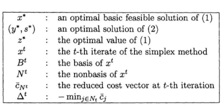
Table 1: Notations

$x^{*}$ : anoptimal basic feasiblesolution of (1)

$(y^{*}, s^{*})$ : anoptimalsolution of (2)

$z^{*}$ : theoptimalvalue of(1)

$x^{t}$ : thet-th iterate of the simplex method

$B^{t}$ : thebasis of$x^{t}$

$N^{t}$ : thenonbasis of$x^{t}$

$\overline{c}_{N^{t},\triangle^{t}}$

: the reduced cost vector at t-thiteration $:$ $- \min_{j\in N_{t}}\overline{c}_{j}$

The coefficient vector $\overline{C}_{N^{t}}=c_{N^{t}}-A_{N^{t}}^{T}(A_{B^{t}}^{-I})^{T}c_{B^{t}}$ is called

a

reduced cost

vector. When $\overline{c}_{N^{t}}\geq 0$, the current solution is optimal. Otherwise

we

conduct

a

pivot. That is,

we

choose

one

nonbasicvariable (entering variable)

and increase the variable until

one

basic variable (leaving variable) becomes

zero.

Then

we

exchange the two variables.

Under the

most negative rule,

we

choose

an

entering variable whose reduced cost is minimum. To put it

precisely,

we

choose

an

index

$j_{MN}^{t}= \arg\min_{j\in N_{t}}\overline{c}_{j}$.

We set $\triangle^{t}=-\overline{C}\cdot t$

$\mathcal{J}_{MN}^{\cdot}$

We summarize the notations in Table 1.

3

Geometric

Interpretation

If

we

write LP inthedictionary form (4), it

can

be

seen as a

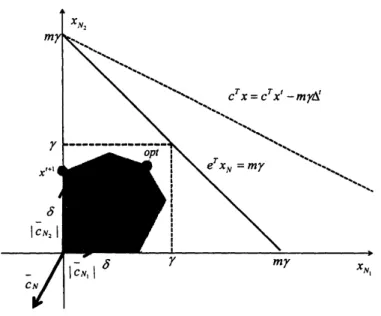
problem in $x_{N^{t}}$

space. The current point $x^{t}$ corresponds to the origin (Figure 1). Assume

that $x^{t}$ is not optimal. Then at least

one

component of the reduced cost $C_{N^{t}}$ is negative. From the definition of

$\delta$ and

$\gamma$, all the BFSs other than

$x^{t}$

are

contained in the square with length $\gamma$ minus the square with length

$\delta$

.

Under the most negative rule,

a

nonbasic variable whose coefficient of the

reduced cost is minimum is chosen

as

the enteringvariable. In Figure 1, $x_{N_{2}}$

is chosen

as

the entering variable. Then the iterate

moves on

the $x_{N_{2}}$ axis.

The objective function decreases $\triangle^{t}=\overline{c}_{N_{2}}$ per unit distance. In this

case

the iterate

moves

at least $\delta$, thus the objective function decreases at least

$\delta\Delta^{t}$. Then

we

get the following inequality.

$c^{T}x^{t+1}\leq c^{T}x^{t}-\delta\triangle^{t}$ (5)

We

go

on

with Figure 1. All the BFSs

are

contained in the set $S=$

$\{x_{N^{t}}|x_{N^{t}}\geq 0, e^{T}x_{N^{t}}\leq m\gamma\}$. Then the intercept of each axis is $m\gamma$. If

we

consider the contour at the intercept of the axis with the minimum

co-efficient (in this

case

$x_{N_{2}}$), the contour passes outside

Figure

1:

The

feasible

region

seen

from

a

nonoptimal

BFS

$x\in S\Rightarrow c^{T}x\geq c^{T}x^{t}-m\gamma\Delta^{t}$ . If

we

take

an

optimal BFS

as

$x$,

we

get the

following lemma.

Lemma 3.1 $[2J$ Let $z^{*}$ be the optimal value

of

Problem (1) and $x^{t}$ be the

t-th itemte generated by the simplex method with the most negative rule.

Then

we

have

$z^{*}\geq c^{T}x^{t}-\triangle^{t}m\gamma$. (6)

By combining (5) and Lemma 3.1, we obtain the following theorem.

Theorem 3.1 [2] Let$x^{t}$ and$x^{t+1}$ be the t-th and_$(t+1)$-thiterates generated

by the simplex method with the most negative rule.

_If

$x^{t+1}\neq x^{t}$, then

we

have

$c^{T}x^{t+1}-z^{*} \leq(1-\frac{\delta}{m\gamma})(c^{T}x^{t}-z^{*})$. (7)

Next we consider a dictionary at an optimal BFS (Figure 2).

$\min$ $c_{B^{*}}^{T}A_{B^{*}}^{-1}b+\overline{c}_{N^{*}}^{T}x_{N^{*}}$,

$s$.$t$ $x_{B^{*}}=A_{B^{*}}^{-1}b-A_{B^{*}}^{-I}A_{N}*x_{N^{*}}\geq 0$,

$x_{N^{*}}\geq 0$

In this case, all the components of the reduced cost $\overline{c}_{N^{*}}$ is nonnegative.

The

gap

between

the

objective value

of

the current iterate $x^{t}$ and $z^{*}$ is

$c^{T}x^{t}-z^{*}=\overline{c}_{N^{*}}^{T}x_{N^{*}}^{t}$ and

we

draw the contour at $x^{t}$

.

Then there exists

an

index $j\in N^{*}$ whose intercept is less than

or

equal to $mx_{j}^{t}$ (in Figure 2, $N_{1}^{*}$

is such

an

index). The contourof$\overline{c}_{N^{*}}^{T}x_{N^{*}}$ is derived by reducingthecontour

at $x^{t}$ by $\frac{c^{T}x-z^{*}}{c^{T}x^{t}-z^{*}}$ times, and the intercept reduces at the

same

rate. Thus

we

Figure 2: Feasible region seen from an optimal BFS

Lemma 3.2 [2] Let $x^{t}$ be the t-th iterate genemted by the simplex method.

If

$x^{t}$ is not optimal, there exists $\overline{j}\in B^{t}$ such that

$x \frac{t}{j}>0$ and

for

any $k$, the k-th itemte $x^{k}$

satisfies

$x \frac{k}{j}\leq\frac{m(c^{T}x^{k}-z^{*})}{c^{T}x^{t}-z^{*}}x\frac{t}{j}$.

Figure 3 is useful to show how

we

obtain the bound for the number of

different basic solutions. If the primal problem (1) is nondegenerate,

we

Figure 3: Changes in $x_{\overline{j}}$

have $x^{t+1}\neq x^{t}$ for all $t$. Then by theorem 3.1, the upper bound of

implied in Lemma

3.2

becomes $m(1- \frac{\delta}{m\gamma})^{k-t}x\frac{t}{j}$. If$k$ is bigger than $k_{0}$, the

upper bound is less than

$\delta$

, meaning

$x \frac{k}{j}$

is

zero

from the definition of

$\delta$

.

More

generally,

we

have the following result.

Lemma 3.3 $f2$] Let$x^{t}$ be the t-th itemte genemted by the simplex method

with the most negative rule.

Assume

that $x^{t}$ is not

an

optimal solution.

Then there exists $\overline{j}\in B^{t}$ satisfying the following two conditions.

1. $x \frac{t}{j}>0$

.

2.

_If

the simplex method genemtes $\lceil m1\log(m)1$

different

basic

feasible

solutions

_afler

t-th itemte, then $x_{\overline{j}}$ becomes

zero

and stays $zem$

.

The event described in Lemma

3.3 can occur

at most

once

for each variable.

Thus

we

get the following result.

Theorem 3.2 [2] When we apply the simplex method withthe most negative

rule

_for

$LP(1)$ having optimalsolutions,

we

encounterat most$n\lceil m_{\delta}^{f}\log(m_{\delta}^{f})\rceil$

different

basic

_feasible

solutions.

Note that the result is valid

even

if the simplex method fails to find

an

optimal solution because of

a

cycling.

Ifthe primal problem is nondegenerate,

we

have$x^{t+1}\neq x^{t}$ for all$t$

.

This

observation leads to

a

bound for the number of iterations of the simplex

method.

Corollary 3.1 $[2J$

If

theprimalproblem is nondegenemte, the simplexmethod

finds

an

optimal solution in at most$n\lceil m_{\delta}^{f}\log(m_{\delta}^{f})\rceil$ itemtions.

4

Applications

to

Special LPs

We havethe following result for

an

LP whose constraint matrix $A$ is totally

unimodularand allthe elements of$b$

are

integers. Recallthat the matrix$A$ is

totally unimodular ifthedeterminant of every nonsingular squaresubmatrix

of $A$ is 1 or-l.

Corollary 4.1 $f2$]

Assume

that the constmint matrix $A$

of

(1) is totally

unimodular and the constmint vector $b$ is integml. When

we

apply the

simplex method with the most negative rule

_for

(1),

we

encounter at most

References

[1] G. B. Dantzig: LinearProgramming andExtensions. Princeton

Univer-sity Press, Princeton, New Jersey, 1963.

[2] T. Kitahara and S. Mizuno: A Bound forthe Number of Different Basic

Solutions Generated by the Simplex Method. Technical report, 2010.

[3] V. Klee and G. J. Minty: How good is the simplex method. In O.

Shisha, editor, Inequalities III, Academic Press, New York, NY,

1972.

[4] Y. Ye: The Simplex Method is StronglyPolynomial for the Markov

De-cision Problem with

a

Fixed Discount Rate. Technical paper, available at http:$//www.stanford.edu/$ yyye$/simplexmdpl.pdf$, 2010.