QUASITORIC MANIFOLDS WHICH ARE NOT TORIC ORIGAMI (The Topology and the Algebraic Structures of Transformation Groups)

QUASITORIC MANIFOLDS WHICH ARE NOT TORIC ORIGAMI

ANTON AYZENBERG,MIKIYA MASUDA,SEONJEONG PARK, ANDHAOZHI ZENG

ABSTRACT. We construct 6-dimensional quasitoric manifolds which are not

toric origamimanifolds.

INTRODUCTION

Origamimanifoldsappearedin differentialgeometry recently

as

a

generalization

of symplectic manifolds [3]. Toric origami manifolds

are

in turn generalizations

of symplectic toric manifolds. Toric origami manifolds

are a

special class of

2n-dimensional compact manifolds with an effective actionofa half-dimensional

com-pact torus $T^{n}$

.

In this paper

we

consider the following question. How large is this

class? Which manifolds with half-dimensional torus actions

are

toric origami

man-ifolds?

Inparticular, whichquasitoric

manifolds

admittoricorigami

structures?

In [7] Masuda and Parkproved

Theorem 1. Anysimplyconnectedcompactsmooth

_4-manifold

$M$ with an

effective

smooth action

_of

$T^{2}$

is equivariantly diffeomorp$hic$ to a toric origami

manifold.

In particular, any 4-dimensional quasitoric manifold is toricorigami. The

same

question about higher dimensions

was

open. Here weprove the negativeresult.

Theorem 2. There exist

6-dimensional

quasitoricmanifolds, which

are

not

equiv-ariantly homeomorphic to any toric origami

_manifold.

We will describe

an

obstruction for

a

quasitoric 6-man 垣 old _{to be toric} origami

and present alarge series ofexamples, where such anobstruction appears. Inspite

oftopological nature of the task, the proof is purely discrete geometrical: it relies

on

metric and coloring properties ofplanar graphs. 1. TOPOLOGICAL PRELIMINARIES

1.1. Quasitoric manifolds. The subject of this subsection originally appeared in the seminal work of Davis and Januszkiewicz [4]. The modern exposition and

technical detailscan be found in [2, Ch.7].

Let $T^{n}$ be

a

compact $n$-dimensional torus. The standard representation of$T^{n}$

is

a

representation $\tau^{n}\sim \mathbb{C}^{n}$ by coordinate-wise rotations. The action of $T^{n}$

on

a

manifold $M^{2n}$ _is called locally standard, if$M$ _has

an

atlas of standard charts,

each isomorphic to

a

subset of the standard representation. In the following $M$ is

supposed to be compact.

Since theorbit space$\mathbb{C}^{n}/T^{n}$ ofthe standard representation isanonnegative

cone

$\mathbb{R}_{\geq}^{n}=\{x\in \mathbb{R}^{n}|x_{i}\geq 0\}$, the orbit space of any locally standard action has the

structure of

a

compactmanifold with

corners.

Let$\mathcal{F}(Q)$ denote the set of facets of$Q$

(i.e. faces of codimension 1). For each facet $F$ of$Q$ consider

a

stabilizer subgroup $\lambda(F)\subset T^{n}$, which preserves points over the interior of $F$

.

This subgroup is 1-dimensional and connected, thus it has the form $\{(t^{\lambda_{1}}, \ldots, t^{\lambda_{n}})|t\in T^{1}\}\subset T^{n}$, for

Thefirst author issupported bythe JSPSpostdoctoral fellowshipprogram. The second author

some primitive integral vector $(\lambda_{1}, \ldots, \lambda_{n})\in \mathbb{Z}^{n}$, defined uniquely up to a common

sign. Thus,

a

primitive integralvector $($uptosign) $\Lambda(F)\in \mathbb{Z}^{n}/\pm is$ associated with

any facet $F$ of $Q$

.

This map $\Lambda:\mathcal{F}(Q)arrow \mathbb{Z}^{n}/\pm is$ called a characteristic

function

(or

a

characteristic map). It satisfies the following so called $(*)$-condition:

Iffacets $F_{1}$, .

.

. ,$F_{s}$ intersect, then the set of vectors

$(*)$

$\Lambda(F_{1})$,

. . .

,$\Lambda(F_{s})$ is

a

part some basis of$\mathbb{Z}^{n}.$

Here

we

actually take not

a

class $\Lambda(F_{i})\in \mathbb{Z}^{n}/\pm$, but

one

of its two particular

representatives in $\mathbb{Z}^{n}$

.

Obviously, the condition does not depend on the choice of sign, thus $(*)$ is well defined. The

same

convention appears further in the text

without special mention.

Definition 1.1. A

_manifold

$M^{2n}$ with a locally standard action

of

$T^{n}$ is called

quasitoric,

_if

the orbit space $M/T^{n}$ is homeomorphic to a simple polytope as a

manifold

with

corners.

Recall that a convex polytope $P$ of dimension $n$ is called simple if any of its

vertices lies in exactly $n$ facets. In other words,

a

simple polytope is

a

polytope

which is at the

same

time

a

manifold with

corners.

Considering manifolds with corners, simple polytopes arethe simplest geometrical examples

one can

imagine. This makes the definition ofquasitoric manifold very natural.

Let $P$ be

a

simple polytope and $\Lambda$ be a characteristic function, i.e. any map

$\Lambda:\mathcal{F}(P)arrow \mathbb{Z}^{n}/\pm$ satisfying ($*)$-condition. The pair $(P, \Lambda)$ is called

a

characteristic

pair. According to [4], there is $a$ one toone correspondence

{quasitoric

manifolds}

$-\{$ characteristic pairs$\}$

up to equivariant homeomorphism on the left-hand side and combinatorial equiva-lence onthe right-hand side. The quasitoric manifold associated with a character-istic pair $(P, \Lambda)$ will be denoted $M_{(P,\Lambda)}$. Let $\eta$ denote the projection to the orbit space $\eta:M_{(P,\Lambda)}arrow P$

.

Each facet $F\in \mathcal{F}(P)$ determines a characteristic

submani-fold $N_{F^{d}}=^{ef}\eta^{-1}(F)\subset M_{(P,\Lambda)}$ of dimension $2n-2$

.

On its own, the manifold $N_{F}$ is

again

a

quasitoric manifold with the orbit space $F.$

1.2. Toric origami manifolds. In the following subsections

we

recall the def-initions and properties of toric origami manifolds and origami templates. More detailed exposition of this theory

can

be found in [3], [7]

or

[6].

A

_folded

symplectic

_form

on a $2n$-dimensional smooth manifold $M$ is a closed

2-form $\omega$ whose top power $\omega^{n}$ vanishes transversally

on a

subset $Z$ and whose

restriction topoints in $Z$has maximal rank. Then $Z$is

a

codimension-one subman-ifold of$M$ called the

fold.

The pair $(M, \omega)$ is called

a

folded

symplectic

manifold.

If $Z$ is empty, $\omega$ is a genuine symplectic form and $(M, \omega)$ is a genuine symplectic

manifold accordingto classical definition.

Sincetherestriction of$\omega$to$Z$ hasmaximalrank, it hasa one-dimensional kernel at each point of $Z$

.

This determines a line field

on

$Z$ called the null

foliation.

If the nullfoliationis the vertical bundle of

some

principal $S^{1}$-fibration$Zarrow Y$

over

a

compact base $Y$, thenthe folded symplectic form $\omega$ is called

an

origami

form

and the pair $(M, \omega)$ is called an origami

manifold.

The action of

a

torus $T$ (of any dimension)

on an

origami manifold $(M, \omega)$ is called Hamiltonian if it admits a moment map $\mu:Marrow t^{*}$ to the dual Lie algebra

ofthe torus, which satisfies the conditions: (1) $\mu$ is equivariant with respect to the

givenactionof$T$

on

$M$_{and the trivial action}of$T$

on

$t^{*};(2)\mu$collectsHamiltonian

functions, that is, $d\langle\mu,$$V\rangle=\omega(V\#$, where $\langle\mu,$$V\rangle$ is the function on $M$, taking

the value$\langle\mu(x)$,$V\rangle$at

a

point$x\in M,$ $V\#$ isavector flowon$M$, generated by$V\in t,$

Definition

1.2.

A toric origami

_manifold

$(M, \omega, T, \mu)$, abbreviated

as

$M$, is

a

compact connectedorigami

_manifold

$(M, \omega)$ equippedwith an

effective

Hamiltonian

action

_of

a torus $T$ with $\dim T=\frac{1}{2}\dim M$ and with

a

choice

of

a $corre\mathcal{S}$ponding

moment map $\mu.$

1.3.

Symplectic

toric

manifolds. When the fold $Z$ is empty,

a

toric origami manifold is

a

symplectic

toric

_manifold.

In this

case

the image$\mu(M)$

of

the moment

map is

a

Delzant polytope in $t^{*}$, and the map

$\mu:Marrow\mu(M)$ itself

can

beidentified

with the map to the orbit space$\eta:Marrow M/T^{n}$

.

A classical theorem of Delzant [5]

says that symplectic toric manifolds are classified by the images of their moment maps in$t^{*}\cong \mathbb{R}^{n}$

.

In other words, there is

a

one-to-one correspondence

{symplectic toric

manifolds}

$-$

{

Delzant

polytopes}

upto equivariant symplectomorphism

on

the left-handside, and affine equivalence on the right-hand side. Let us recall the notion of Delzant polytope.

Definition 1.3. A simple

convex

polytope $P\subset \mathbb{R}^{n}$ is calledDelzant,

if

its normal

fan

is smooth (with respect to a

_fixed

lattice $\mathbb{Z}^{n}\subset \mathbb{R}^{n}$).

Construction

1.4

(Topological model of symplectic toric manifold). Let $P$ be

a

Delzant polytope in$\mathbb{R}^{n}$

.

For

a

facet_{$F\in \mathcal{F}(P)$}consider its outwardprimitivenormal vector $\tilde{\nu}(F)\in \mathbb{Z}^{n}$

.

Consider the corresponding vector modulo $sign:\nu(F)\in \mathbb{Z}^{n}/\pm.$

By the definition ofDelzant polytope, $\nu:\mathcal{F}(P)arrow \mathbb{Z}^{n}/\pm$ satisfies ($*)$, thus provides

an

example of a characteristic function. The quasitoric manifold

$M_{P}^{d}=^{ef}M_{(P,\nu)}.$

is the symplectic toric manifold correspondingto $P$ (up to equivariant

homeomor-phism).

1.4. Origami templates. To generalize Delzant correspondence to toric origami manifolds we need a notion ofan origami template, which

we

review next.

Let $\mathcal{D}_{n}$ denotetheset of all (full-dimensional) Delzant polytopes in

$\mathbb{R}^{n}$ (w.r.t.

$a$

fixed

lattice) and $\mathcal{F}_{n}$ the set of all their

facets.

Definition 1.5. An origami template is a triple $(\Gamma, \Psi_{V}, \Psi_{E})$, where

$\bullet$ $\Gamma$ is a connected

finite

graph (loops and multiple edges are allowed) with the vertex set $V$ and edge set$E_{j}$

$\bullet\Psi_{V}:Varrow \mathcal{D}_{n}$;

$\bullet\Psi_{E}:Earrow \mathcal{F}_{n}$;

subject to the following conditions:

1.

_If

$e\in E$ _is an _edge

of

$\Gamma$ with endpoints

$v_{1},$$v_{2}\in V$, then $\Psi_{E}(e)$ is a

facet

of

bothpolytopes$\Psi_{V}(v_{1})$ and$\Psi_{V}(v_{2})$, and thesepolytopes coincide near$\Psi_{E}(e)$

(this

means

there exists an open neighborhood$U$

of

$\Psi_{E}(e)$ in$\mathbb{R}^{n}$

such that

$U\cap\Psi_{V}(v_{1})=U\cap\Psi_{V}(v_{2}))$

.

2.

_If

$e_{1},$$e_{2}\in E$

are

two edges

of

$\Gamma$ adjacent to$v\in V$, then $\Psi_{E}(e_{1})$ and$\Psi_{E}(e_{2})$

are

disjoint

_{facets of}

$\Psi_{V}(v)$

.

The

_{facets of}

the

_form

$\Psi_{E}(e)$

for

$e\in E$ are called the

fold facets

of

the origami

template.

For convenience in the following we call the vertices of graph $\Gamma$ the nodes.

One

can

simply view

an

origami template

as a

collection of(possibly overlapping) Delzant polytopes $\{\Psi_{V}(v)|v\in V\}$ in the

same

ambient space, with

some

gluing

FIGURE 1. Examplesof origami templates in$\dim=2$

.

Foldfacets

are

shown in red.

Theorem 3 ([3]). Assigning the

moment

data

_of

a

toric origami

_manifold

induces

$a$

one-to-one

correspondence

{toric

origami

manifolds}

$-$

{

origami

templates}

up to equivariant origami symplectomorphism

on

the

_left-hand

side, and

_affine

equivalence on the right-hand side.

Construction 1.6 (Topological construction oftoric origami manifold). Consider

an

origami template $O=(\Gamma, \Psi_{V}, \Psi_{E})$, $\Gamma=(V, E)$

.

Foreachnode$v\in V$ the Delzant

polytope$\Psi_{V}(v)\in \mathcal{P}_{n}$givesasymplectic toricmanifold$M_{\Psi_{V}(v)}$,

see

construction

1.4.

Now do the following procedure:

1 Take adisjoint union ofall manifolds $M_{\Psi_{V}(v)}$ for $v\in V$;

2 For each edge $e\in E$ _{with distinct}endpoints $v_{1}$ and $v_{2}$ takean equivariant

connected

sum

of $M_{\Psi_{V}(v_{1})}$ and $M_{\Psi_{V}(v_{2})}$ alongthe characteristic

submani-fold $N_{\Psi_{E}(e)}$ (whichis embedded in both manifolds);

3 For each loop $e\in E$ based at $v\in V$ take a real blow up of normal bundle

tothe submanifold $N_{\Psi_{E}(e)}$ inside $M_{\Psi_{V}(v)}.$

Step 2 makes

sense

because of pt.1 of Definition 1.5. Indeed, the polytopes

$\Psi_{V}(v_{1})$ and $\Psi_{V}(v_{2})$ agree near $\Psi_{E}(e)$, thus $M_{\Psi_{V}(v_{1})}$ and $M_{\Psi_{V}(v_{2})}$ have

equivari-antly homeomorphic neighborhoods around $N_{\Psi_{E}(e)}$, so the connected sum is well

defined. Pt. 2 ofDefinition 1.5

ensures

that surgeries do not touch each other, so all the connected

sums

and blow ups

can

be taken simultaneously.

Denote the resulting manifold of this construction by$M_{O}=M_{(\Gamma,\Psi_{V},\Psi_{E})}$

.

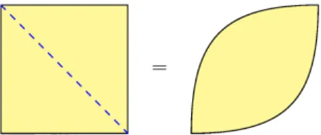
This isexactly the toric origami manifold associated with $O$ via Theorem 3.

Example 1.7. Let

us

construct

a

toric origami manifold $X$, corresponding to the

origami template, made of two triangles (Fig. 1, left). The symplectic toric 4-manifold corresponding to

a

triangle is known to be the complex projective plane

$\mathbb{C}P^{2}$. The

characteristic submanifoldcorrespondingtothe fold facet is

a

projective line $\mathbb{C}P^{1}\subset \mathbb{C}P^{2}$

.

Thus, _$X$is

a

connected

sum

of two copies of $\mathbb{C}P^{2}$ along the line $\mathbb{C}P^{1}$, which lies in both. It is easily

seen

that this manifold is $S^{4}.$

An origami template $O=(\Gamma, \Psi_{V}, \Psi_{E})$ (and the corresponding manifold $M_{O}$)

is called co\"orientable if $\Gamma$ has

no

loops (i.e. edges based at

one

point). If_{$M_{O}$} is co\"orientable, then the action of$T^{n}$ on $M_{O}$ is locally standard [6, lemma 5.1]. The

converse

is also true. In the following we consider only co\"orientabletemplates and toric origamimanifolds.

Construction 1.8 (Orbit space of toric origami manifold). The orbit space $Q=$

$M_{(\Gamma,\Psi_{V},\Psi_{E})}/T^{n}$of$a$ (co\"orientable) toricorigamimanifold isamanifold withcorners.

fold facets. More precisely,

(1.1) $Q=v\in V\sqcup(v, \Psi_{V}(v))/\sim,$

where $(u, x)\sim(v, y)$ ifthere exists

an

edge $e$ with endpoints $u$ and $v$, and _$x=y\in$

$\Psi_{E}(e)$

.

Facets of$Q$ are given by non-fold facets of polytopes $\Psi_{V}(v)$ identified in the

same

way. Tomake thisprecise, let

us

callnon-fold facets $F_{1}\in \mathcal{F}(\Psi_{V}(v_{1}))$ and $F_{2}\in \mathcal{F}(\Psi_{V}(v_{2}))$ elementary neighboring w.r.$t$. to the edge $e\in E$ (withendpoints

$v_{1}$ and $v_{2}$) if$F_{1}\cap\Psi_{E}(e)=F_{2}\cap\Psi_{E}(e)$

.

The relation ofelementary neighborliness

generates

an

equivalence relation $rightarrow on$thesetofall non-fold facets ofallpolytopes

$\Psi_{V}(v)$

.

Define the facet $[F]$ of the orbit space $Q$

as a

union of facets in

one

equivalence class:

(1.2) $[F] def= \sqcup(v, G)/\sim, [F]\in \mathcal{F}(Q)$,

$Gisnotf\circ 1d,Grightarrow Fv\in V,G\in \mathcal{F}(\Psi_{V}(v)),$

where $\sim$ isthe

same as

in (1.1).

Letus define aprimitive normal vectorto the facet $[F]$ of$Q$ by $v([F])^{d}=^{ef}\nu(F)\in$

$\mathbb{Z}^{n}/\pm$

.

It is welldefined since $\nu(F)=\nu(G)$ for $Frightarrow G.$

Note that therelation ofelementary neighborlinessdetermines

a

connected sub-graph$\Gamma_{[F]}$ of$\Gamma$

.

Allfacets$Grightarrow F$

are

Delzant and lie in the

same

hyperplane_{$H_{[F]}.$}

Thus

we

obtain

an

induced origami template

(1.3) $O_{[F]}=(\Gamma_{[F]}, \Psi_{V}|_{\Gamma_{[F]}}\cap H_{[F]}, \Psi_{E}|r_{[F]}\cap H_{[F]})$

ofdimension $n-1$

.

In particular, if$\eta:M_{O}arrow Q$ denotes the projection to the orbit

space, then the characteristic submanifold $\eta^{-1}([F])$ is the toric origami manifold

ofdimension $2n-2$ generated by the origami template $O_{[F]}.$

Extendingtheorigami analogy,

we can

think of the orbit space$Q$ as“unfolding” the origami template and then smoothening the angles adjacent to the former

fold

facets (remember that

we

haveto identify neighboring faces!).

FIGURE 2. The orbit space of amanifold $S^{4}$, corresponding to the

origami template shownon Fig. 1, left.

It is easyto

see

that the orbit space $Q=M_{(\Gamma,\Psi_{V},\Psi_{E})}/T^{n}$ hasthe

same

homotopy

type

as

the graph $\Gamma$, thus _$Q$ is either contractible (when $\Gamma$ is

a

tree)

or

homotopy equivalentto

a

wedgeofcircles. Thisobservationshows that whenever the template graph$\Gamma$ has cycles, the corresponding toric origami manifold cannot be quasitoric.

As

an

example, the origami template shown

on

Fig. 1, at the right corresponds to

the origami manifold which is not quasitoric. Since we want to find a quasitoric

manifold which is not toric origami,

we

need to consider only the

cases

when the orbit space is contractible. Thus in the following $\Gamma$ is supposed to be

a

tree.

2. WEIGHTED SIMPLICIAL SPHERES

In the previous section

we

have seen that quasitoric manifolds

are

encoded by the orbit spaces (which

are

simple polytopes) and characteristic functions (which

are

colorings of facets by elements of $\mathbb{Z}^{n}/\pm$). It will be easier, however, to work

with the dual objects, which we call weighted simplicial spheres.

Recall that a simplicial poset is a finite partially ordered set $S$ such that: (1)

There is

a

unique minimal element $\emptyset\in S$, (2) For each $I\in S$ the interval subset $[\emptyset, I]def=\{J\in S|J\leq I\}$ _{is isomorphic to the poset} of faces of _$(k-1)$-dimensional

simplex (i.e. Boolean lattice ofrank $k$). In this

case

the element $I$ is saidto have

rank $k$ and dimension $k-1$. The elements of$S$

are

called simplices and elements

of rank 1 are called vertices. The set ofvertices of$S$ is denoted Vert(S).

A simplicial poset is called pure, if all maximal simplices have the same

dimen-sion. Asimplicial poset $S$ is called

a

simplicial complex, iffor any subset ofvertices $\sigma\subseteq Vert(S)$, there exists at most

one

simplex whose vertex set is $\sigma.$

Construction 2.1. It is convenient to visualize simplicial posets using their geo-metrical realizations. Assign the geogeo-metrical simplex $\Delta_{I}$ of dimension rank$(I)-1$ to each $I\in S$ andattach them together according to the order relation in $S$

.

More

formally, the geometric realization of$S$is the topological space

$|S|^{d}=^{ef}\sqcup(I, \triangle_{I})/\sim I\in S$’

where $(I_{1}, x_{1})\sim(I_{2}, x_{2})$ if$I_{1}<I_{2}$ and $x_{1}=x_{2}\in\Delta_{I_{1}}\subset\Delta_{I_{2}}$

.

See details in [2].

A simplicial poset $S$ is called atriangulated sphere if $|S|$ is homeomorphic to a

sphere. $S$ is called

a

PL-sphere if the barycentric subdivision $S’$ (which is a

sim-plicial complex) is PL-homeomorphic to the boundary ofa simplex. In dimension 2, which istheonly important

case

for us, these two notions

are

equivalent. Inthe sequel

we

call either of them simplicial spheres.

Construction 2.2. Let us define a connected sum oftwo simplicial spheres along

their vertices. At first we should exclude certain degenerate situations.

For every

$I<J$

in $S$ there is a complementary simplex $J\backslash I\in S$

.

In other

words, $J\backslash I$ is the face of $J$ complementary to the face $I$. Define a link of a

simplex $I\in S$

as a

_{partially ordered set} $1ink_{S}I=\{J\backslash I|J\in S, J\geq I\}$ with

the order relation induced from $S$

.

Define an open star of a simplex $I\in S$

as

a

subset $star_{S}^{o}$$I$ $def=\{J\in S|J\geq I\}$

.

There is a natural surjective map of sets

$D_{I}:star_{S}^{o}Iarrow 1ink_{S}$$I$ sending $J$ to $J\backslash I$

.

We call a simplex I admissible if$D_{I}$ is

injective.

Note that in a simplicial complex every simplex is admissible. One can view

admissibility as the propertyof being “locally a simplicial complex

Let us define theconnectedsum oftwo simplicial posets $S_{1}$ and$S_{2}$ along

admis-sible vertices. Let $i_{1}\in S_{1}$ and $i_{2}\in S_{2}$ be admissible vertices, and suppose there

exists

an

isomorphism ofposets $\xi:1ink_{S_{1}}i_{1}arrow 1ink_{S_{2}}i_{2}$ (thus an isomorphism of open stars, by admissibility). Consider

a

poset

(2.1) $S_{1i_{1}}\#_{i_{2}}S_{2}^{d}=^{ef}(S_{1}\backslash star_{\mathring{S}_{1}}i_{1})\sqcup(S_{2}\backslash star_{S_{2}}^{o}i_{2})/\sim,$

where $I_{1}\in 1ink_{S_{1}}i_{1}\subset S_{1}$ is identifiedwith $I_{2}\in 1ink_{S_{2}}i_{2}\subset S_{2}$ whenever $I_{2}=\xi(I_{1})$

.

The order relation

on

$S_{1i_{1}}\#_{i_{2}}S_{2}$ is induced from $S_{1}$ and $S_{2}$ in a natural way. The

poset $S_{1i_{1}}\# i_{2}S_{2}$ is simplicial. If$S_{1},$$S_{2}$

are

simplicial spheres, then

so

is $S_{1i_{1}}\#_{i_{2}}S_{2}$

(this property may break for non-admissible vertices).

Definition 2.3. Let $S$ be a pure simplicial poset

of

dimension $n-1$

.

A map $\Lambda:Vert(S)arrow \mathbb{Z}^{n}/\pm is$ called a weighting if,

for

every simplex $I\in S$ with vertices

$i_{1}$,

.

.

.

,$i_{n}$, the vectors$\Lambda(i_{1})$, .

. .

,$\Lambda(i_{n})$ span$\mathbb{Z}^{n}$

.

Thepair $(S, \Lambda)$ is called aweighted

simplicial poset.

Definition 2.4. Let $(S_{1}, \Lambda_{1})$ and $(S_{2}, \Lambda_{2})$ be weighted simplicial posets. Let$i_{1},$$i_{2}$

$1ink_{S_{2}}i_{2}$ preserving weights: $(\Lambda_{2}\circ\xi)|_{1inks_{1}^{i_{1}}}=\Lambda_{1}|_{1ink_{S_{1}}i_{1}}$

.

Then $\Lambda_{1},$$\Lambda_{2}$ induce the weight $\Lambda$

on the connected sum$S_{1i_{1}}\# i_{2}S_{2}$

.

The weighted simplicial poset $(S_{1i_{1}}\#_{i_{2}}$

$S_{2},$$\Lambda)$ is called a weighted connected

sum

of

$(S_{1}, \Lambda_{1})$ and $(S_{2}, \Lambda_{2})$

.

Construction 2.5. Let $(P, \Lambda)$ be a characteristic pair (see section 1). Let $K_{P}=$

$\partial P^{*}$ be the dual simplicial sphere to

a

simple polytope _$P$

.

Since there is

a

natural correspondence Vert$(K_{P})=\mathcal{F}(P)$

we

get the weighting $\Lambda:Vert(K_{P})arrow \mathbb{Z}^{n}/\pm.$ This defines

a

weighted sphere $(K_{P}, \Lambda)$

.

In particular, any Delzant polytope $P$ defines aweighted sphere $(K_{P}, \nu)$, where $\nu(F)$ is the normal vector to$F\in \mathcal{F}(P)=$

$Vert(K_{P})$ modulo_{sign (construction 1.4).}

Construction

2.6.

Let $O=(\Gamma, \Psi_{V}, \Psi_{E})$ be

an

origami template and $M_{O}$ be the

corresponding toric origami manifold. Suppose that $\Gamma$

is

a

tree. The orbit

space

$Q=M_{O}/T^{n}$ is homeomorphic to

an

$n$-dimensional disc. The face structure of$Q$ defines a poset $S_{Q}$, whose elements

are

faces of $Q$ ordered by reversed inclusion

(it is easy to show that such poset is simplicial). In particular, Vert$(S_{Q})=\mathcal{F}(Q)$

.

Normal vectorsto facets of$Q$ (construction 1.8) determine the characteristic

func-tion $\nu:\mathcal{F}(Q)arrow \mathbb{Z}^{n}/\pm,$ _{$\nu([F])=\nu(F)$}

.

Thus there is

a

weighted simplicial poset

$(S_{Q}, \nu)$ associated with

a

toric origami manifold $M_{O}.$

Construction

2.7.

If $\Gamma$ is

a

tree, then the simplicial poset

$S_{Q}$ is the connected

sum

ofsimplicial spheres $K_{\Psi_{V}(v)}$ alongvertices, corresponding to fold facets:

(2.2) $S_{Q}\cong\# K_{\Psi_{V}(v)}\Gamma^{\cdot}$

Let

us

introduce

a

notation to make this precise. Let $e$ be

an

edge of $\Gamma$, and

$v$ be its endpoint. Let $i_{v,e}$ be the vertex of $K_{\Psi_{V}(v)}$ corresponding to the facet

$\Psi_{E}(e)\subset\Psi_{V}(v)$

.

Then (2.2) denotes the connected

sum

of all simplicial spheres

$K_{\Psi_{V}(v)}$ alongvertices$i_{v,e},$$i_{u,e}$for alledges$e=\{v, u\}$ofgraph$\Gamma$

.

This simultaneous connected

sum

is well defined. Indeed, if $e_{1}\neq e_{2}\in E$

are

two edges emanating

from $v\in V$, then vertices $i_{v,e_{1}}$ and $i_{v,e_{2}}$

are

not adjacent in $K_{\Psi_{V}(v)}$ by pt.2 of

Definition 1.5. Therefore, open stars$star_{K_{\Psi_{V}(v)}}^{o}i_{v,e_{1}}$ and $star_{K_{\Psi_{V}(v)}}^{o}i_{v,e_{2}}$, which

we

remove

in (2.1), do not intersect. Also note that all vertices $i_{v,e}$

are

admissible,

since the spheres $K_{\Psi_{V}(v)}$

are

simplicial complexes.

Each sphere $K_{\Psi_{V}(v)}$

comes

equipped with a weighting $v_{v}:Vert(K_{\Psi_{V}(v)})arrow$

$\mathbb{Z}^{n}/\pm$, since $\Psi_{V}(v)$ is Delzant. By pt.1 of Definition 1.5 these weightings agree on identified links. Therefore we have an isomorphism of weighted spheres

(2.3) $(S_{Q}, v)\cong\#(K_{\Psi_{V}(v)}, \nu_{v})\Gamma^{\cdot}$

3. PROOF OF THEOREM 2

Suppose that

a

quasitoric manifold $M_{(P,\Lambda)}$ is equivariantly homeomorphic to

the origami manifold $M_{(\Gamma,\Psi_{V},\Psi_{E})},$ $\Gamma$ is

a

tree. First, the orbit spaces should be

isomorphic

as

manifolds with

corners:

$P\cong Q=M_{O}/T^{n}$

.

Second, $M_{(P,\Lambda)}\cong T$

$M_{O}$ implies that stabilizers of the torus actions coincide for the corresponding faces of orbit spaces. Thus characteristic functions

on

$P$ and $Q$ taking values in

$\mathbb{Z}^{n}/\pm are$ the

same.

Hence, the weighted simplicial spheres $(K_{P}, \Lambda)$ and $(S_{Q}, \nu)\cong$

$\#_{\Gamma}(K_{\Psi_{V}(v)}, \nu)$

are

isomorphic. So far to prove Theorem 2 it is suficientto prove

Proposition 3.1. There exists asimple 3-dimensional polytope$P$ and a

character-istic

_function

$\Lambda:\mathcal{F}(P)arrow \mathbb{Z}^{3}/\pm such$ that the dual weighted sphere $(K_{P}, \Lambda)$ cannot

be representedas a connected sum, along atree,

_of

weighted spheres dual to Delzant polytopes.

We proceed by steps. At first notice that any simplicia12-sphere, which is a simplicial complex, is dual to

some

simple 3-polytope by Steinitz’s theorem (see e.g. [10]). Thus it is sufficient to prove the statement for weighted simplicial complexes-spheres of dimension 2.

FIGURE

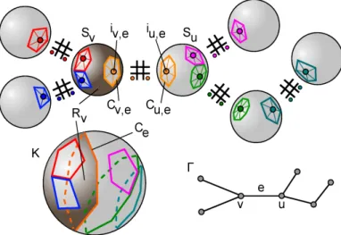
3.

Connected

sum

ofspheres along

a

tree

Construction 3.2. We introduce

some

notation in addition to that of construc-tion 2.7,

see

Fig. 3. As before, let $\Gamma=(V, E)$ be a tree. Suppose that a simplicial

$(n-1)$-sphere $S_{v}$ is associated with each node$v\in V$, and for each edge $e\in E$ with

an endpoint $v\in V$ _{there is} an _{admissible vertex} $i_{v,e}\in S_{v}$ subject to the following

conditions: (1) $1ink_{S_{v}}i_{v,e}$ is isomorphic to $1ink_{S_{u}}i_{u,e}$ for any edge $e$ with endpoints

$v,$$u;(2)$ Vertices $i_{v,e_{1}},$$i_{v,e_{2}}$ are different and not adjacent in $S_{v}$ for any twoedges

$e_{1}\neq e_{2}$ emanating from $v$

.

Then

we can

form

a

connected

sum

along $\Gamma$

as

in construction 2.7: $K=\#_{\Gamma}S_{v}$

.

For each $v\in V$ considerthe simplicial subposet

(3.1) $R_{v}=S_{v}\backslash _{e\in E}\sqcup_{v\in e}star_{S_{v}}^{o}i_{v,e}.$

This subposet will be called

a

region. Denote $1ink_{S_{v}}i_{v,e}$ by $C_{v,e}$. By construction, $C_{v,e}$ is attached to $C_{u,e}$ if$e=\{v, u\}$

.

The resulting $(n-2)$-dimensional simplicial

subposetof$K$is denoted by$C_{e}$

.

Since$i_{v,e}$ is admissible, the subposet $C_{e}\cong C_{v,e}=$

$1ink_{S_{v}}i_{v,e}$ is asimplicial $(n-2)$-sphere.

Weget a collection of$(n-2)$-dimensional cycles $C_{e},$$e\in E$, dividing the $(n-1)-$

sphere $K$ into regions $R_{v},$$v\in V$

.

If $e=\{v, u\}$, then $R_{v}$ and $R_{u}$ share a common

border $C_{e}$. Note that cycles $C_{e}$

are

mutually ordered, meaning that each $C_{e}$ lies

at

one

side of any other cycle. Though the cycles may have

common

points (as schematically shown

on

Fig. 3) and

even

coincide (in this

case

the region between them coincides withboth ofthem).

Ontheotherhand, anycollectionofmutuallyordered $(n-2)$-dimensional spher-ical cycles in $K$ defines the representation of $K$ as a connected sum of smaller

simplicial spheres. A representation $K=\#{}_{\Gamma} S_{v}$ will be called a slicing.

Define the width of a slicing $\Theta$ to be the maximal number of vertices in its regions:

(3.2) wid$( \Theta)^{d}=^{ef}\max\{|$Vert$(R_{v})||v\in V\}.$

Definethe

_fatness

ofa sphere$K$ as_{the minimal width of all its possible} slicings:

The essential step inthe proof of Proposition

3.1

is the following.

Lemma 3.3. Let$K$ be an_$(n-1)$-dimensionalsimplicial sphere and$\Lambda:Vert(K)arrow$

$\mathbb{Z}^{n}/\pm a$ weighting. Let $r$ denote the number

of

different

values

of

this weighting,

$r=|\Lambda(Vert(K))|$

.

Suppose that $ft(K)>2r$

.

Then $(K, \Lambda)$

cannot

be represented

as

a

connected sum, along a tree,

_of

simplicial spheres dual to Delzant polytopes.

Proof.

Assume the

converse.

Then $(K, \Lambda)\cong\#_{\Gamma}(K_{\Psi_{V}(v)}, \nu_{v})$, where $\Psi_{V}(v)$

are

Delzant polytopes. Ifweforget the weights, thisdefines

a

slicing$\Theta$of_$K$

.

Thewidth

of every slicing of $K$ is greater than $2r$ by the definition offatness. In particular,

$wid(\Theta)>2r$

.

_{Thus there exists}

a

node $v$ of$\Gamma$ such that

$|Vert(R_{v})|>2r.$

The region $R_{v}$ is

a

subcomplex of $K_{\Psi_{V}(v)}$

.

The restriction of $\Lambda$ to the subset Vert$(R_{v})$ coincides with the restriction of $\nu:Vert(K_{\Psi_{V}(v)})arrow \mathbb{Z}^{n}/\pm toVert(R_{v})$

.

Recall, that $\tilde{\nu}(F)\in \mathbb{Z}^{n}$ is theoutward normal vector to the facet $F\in \mathcal{F}(\Psi_{V}(v))=$

Vert$(K_{\Psi_{V}(v)})$, and $\nu(F)\in \mathbb{Z}^{n}/\pm is$ its class modulo sign. The outward normal

vectors to facets of

a

convex

polytope

are

mutually distinct, thus $|\tilde{\nu}($Vert R $)|=$

$|Vert(R_{v})|$ and, therefore, $|\nu(Vert(R_{v}))|\geq|Vert(R_{v})|/2$

.

Thus $|\Lambda(Vert(R_{v}))|=$

$|\nu(Vert(R_{v}))|>r$, – the contradiction, since $r$ is the total number of values of$\Lambda.$ $\square$

So far we may find counterexamples to origami realizability among polytopes, which

are

$\mathbb{Z}^{n}$-colored with a small number of colors, but whose dual simplicial spheres have large fatness. Of

course

such examples do not exist for $n=2$ –

this would contradict Theorem 1. The existence of2-spheres satisfying conditions of Lemma

3.3

is thus

our

next and primary goal. At first, we prove that any 2-sphere admitsa characteristic functionwithfew values; then construct 2-spheres of arbitrarilylarge fatness.

Lemma 3.4. Any simplicial 2-sphere $K$ admits a weighting $\Lambda:Vert(K)arrow \mathbb{Z}^{3}/\pm$ such that $|\Lambda(Vert(K))|\leq 4.$

Proof.

Fourcolortheoremstates that there exists

a

proper vertex-coloring: Vert$(K)arrow$

$\{\alpha_{1}, \alpha_{2}, \alpha_{3}, \alpha_{4}\}$

.

Nowreplacecolorsby integral vectors$\alpha_{1}\mapsto(1,0,0)$, $\alpha_{2}\mapsto(0,1,0)$, $\alpha_{3}\mapsto(0,0,1)$, $\alpha_{4}\mapsto(1,1,1)$

.

This gives the required characteristic function. $\square$ Proposition 3.5. For any $N>0$ there exists a simplicial 2-sphere $K$ such that

$ft(K)>N.$

Proof

Construction 3.6. Let$K$be

a

simplicia12-comp1ex. Define$a$(piecewise

Riemann-ian) metric $g$ and

measure

$\mu$

on

$|K|$ in such a way that eachtriangle $|I|\subset|K|$

be-comes an

equilateralEuclidiantrianglewith thestandard metric and edge length 1. Thus the area of each triangle is $\sqrt{3}/4.$

Let $L(\gamma)$ denote the length of

a

piecewise smooth

curve

$\gamma$ in $|K|$

.

If$C\subset K$ is

a

closed 1-dimensional cycle (simplicial subcomplex), then, obviously,

(3.4) $L(|C|)=|Vert(C)|.$

A cycle $C$ divides $K$ into two subcomplexes _{$K+andK_{-}$}, each homeomorphic to

a closed 2-disc (we suppose $C\subset K_{+},$$K$ Let us estimate the number ofvertices

in $K_{-}$ in terms ofits

area

($K_{+}$ is similar). Let $\mathcal{V}_{-},$$\mathcal{E}_{-},$$\mathcal{T}$-denote the number of

vertices, edges and triangles in$K_{-}$

.

By thedefinition ofmeasure, $\mathcal{T}_{-}=\frac{4}{\sqrt{3}}\mu(|K_{-}|)$

.

We have$\mathcal{V}_{-}-\mathcal{E}_{-}+\mathcal{T}_{-}=1$ (Euler characteristic of$K_{-}$) and $\mathcal{E}_{-}<3\mathcal{T}_{-}$ (bycounting

pairs $e\subset t$, where $e$ is

an

edge and $t$ is

a

triangle). Therefore,

Let$\mathbb{S}_{R}$ be

a

2-dimensional round sphereof radius $R$, with the standard metric $g_{s}$

and

measure

$\mu_{s}$. Apiecewisesmoothclosed curve$\gamma\subset \mathbb{S}_{R}$ withoutself-intersections

divides $\mathbb{S}_{R}$ into two regions $A_{+},$ $A_{-}$

.

The isoperimetric inequality

on

asphere (see

e.g. [8, Ch.4]) hasthe form$R^{2}L_{s}(\gamma)^{2}\geq\mu_{s}(A_{+})\mu_{s}(A_{-})$, where$L_{s}(\gamma)$ isthe lengthof

$\gamma$

.

Since $\mu_{s}(\mathbb{S}_{R})=4\pi R^{2}$

we

may

assume

that $\mu_{s}(A_{+})\geq 2\pi R^{2}$ (otherwise consider

$A_{-}$ instead), thus

(3.6) $\mu_{\mathcal{S}}(A_{-})\leq\frac{L_{s}(\gamma)^{2}}{2\pi}.$

Let $K$ be a 2-dimensional simplicial sphere and $R,$$c_{1},$$c_{2},$$c_{3},$$c_{4}$ be positive real

numbers. Suppose thereexists abijective piecewise smooth map$f:|K|arrow \mathbb{S}_{R}$ such that

(3.7) $c_{1}L(\gamma)\leq L_{s}(f(\gamma))\leq c_{2}L(\gamma)$,

(3.8) $c_{3}\mu(\Omega)\leq\mu_{s}(f(\Omega))\leq c_{4}\mu(\Omega)$,

for each piecewise smooth curve $\gamma\subset|K|$ and measurable set $\Omega\subset|K|$

.

Numbers

$c_{1},$$c_{2},$$c_{3},$$c_{4}$ will be called Lipschitz constants ofthe map $f.$

Lemma

3.7.

In the above setting, suppose the cycle $C\subset K$ contains at most $N$

vertices. Then either$K_{+}$

or

$K_{-}$ contains at most

$\underline{4N^{2}c^{2}}$

vertices.

$\sqrt{3}\pi c_{3}$

Proof.

Among two regions $f(|K_{-}|)$,$f(|K+|)\subset \mathbb{S}_{R}$ let $f(|K_{-}|)$ be the

one

with the

smaller

area.

Combine (3.4), (3.5), (3.6), (3.7), and (3.8):

(3.9) $V_{-} \leq\frac{8}{\sqrt{3}}\mu(|K_{-}|)\leq\frac{8\mu_{s}(f(|K_{-}|))}{\sqrt{3}c_{3}}\leq\frac{8L_{s}(f(|C|))^{2}}{2\sqrt{3}\pi c_{3}}\leq\frac{4N^{2}c_{2}^{2}}{\sqrt{3}\pi c_{3}}.$

$\square$ Lemma 3.8.

_If

$\Theta$

is aslicing$K=\#_{\Gamma}S_{v}$ and$wid(\Theta)\leq N$, then$\deg v\leq 2(N-2)$

for

any node $v$

of

$\Gamma.$

Proof.

Denote the degree of$v$ by $d$

.

By construction, the region $R_{v}$ is obtained

from a sphere $S_{v}$ by removing $d$ open stars which correspond to the edges of $\Gamma$ emanating from $v$

.

The complex $R_{v}$ itself

can

be considered

as

a plane graph.

Denote thenumbers ofitsvertices, edges and faces by$\mathcal{V},$$\mathcal{E},$$\mathcal{R}$ respectively. By the

definition of thewidth, we have $\mathcal{V}\leq N$. We also have $\mathcal{V}-\mathcal{E}+\mathcal{R}=2$, and $2\mathcal{E}\geq 3\mathcal{R}$

(each region has at least 3 edges). Thus, $\mathcal{V}\geq 2+\frac{1}{2}\mathcal{R}$

.

Notice that each removed

openstar representsafaceofgraph$R_{v}$, therefore, $d\leq \mathcal{R}\leq 2(\mathcal{V}-2)\leq 2(N-2)$

.

$\square$ Lemma 3.9. Let $K$ be a 2-dimensional simplicial sphere endowed with the map

$f$ to the round sphere, satisfying Lipschitz bounds (3.7) and (3.8). For a natural

number $N$ set $A= \frac{4N^{2}c^{2}}{\sqrt{3}\pi c_{3}}$ and

$B=2(N-2)$

.

If

$| Vert(K)|>\max(AB+N, 2A)$,

then$ft(K)>N.$

Proof.

Assume the contrary: $ft(K)\leq N$

.

Then there is a slicing $K=\#_{\Gamma}S_{v}$ in

which every region $R_{v}$ has at most $N$ vertices. Consequently, any cycle $C_{e},$$e\in E$

has at most $N$ vertices. By Lemma 3.7, the cycle $C_{e}$ divides $K$intotwo parts, one

ofwhich has $\leq A$ vertices. Since _{$|Vert(K)|>2A$}, the other part has $>A$ vertices. Assign a direction to eachedge $e$ of$\Gamma$ in such

a

way that

$e$ points fromthe larger

componentof$K\backslash C_{e}$ tothe smaller, where the siz$e’$

means

thenumber ofvertices,

$\Gamma$ is a tree, therefore there exists a source _$u$, i.e. a node from which all

adja-cent edges emanate. Let $d$ denote the degree of $u$ and $\Gamma_{1}$,.

.

.,$\Gamma_{d}$ the connected

components of $\Gamma\backslash u$

.

By Lemma 3.8 we have $d\leq B$. By the construction

of the directions of edges, $|Vert(\sqcup_{\Gamma_{i}}R_{v})|\leq A$ for each $\Gamma_{i}$

.

Thus $|Vert(K)|<$

Lemma

3.10.

For any $N>0$ there exists

a

2-dimensional simplicial sphere $K$

such that:

(1) There exists a piecewise smooth map $f:|K|arrow \mathbb{S}_{R}$ satisfying Lipschitz

bounds (3.7) and (3.8)

_for

some constants$c_{1},$$c_{2},$$c_{3},$ $c_{4},$$R>0$

(2) $| Vert(K)|>\max(AB+N, 2A)$, where $A$ and$B$ are

defined

in Lemma 3.9.

Proof.

Start

with the boundary of

a

regular tetrahedron with edge length 1: $L=$ $\partial\Delta^{3}$

.

The projection from the center of$L$to the circumsphere $f:Larrow \mathbb{S}_{R}$ is

obvi-ously Lipschitz for

some

constants $c_{1},$$c_{2},$$c_{3},$$c_{4}>0$

.

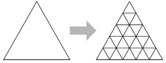
Now subdivide eachtriangleof

$|L|$ into $q^{2}$ smaller regular triangles

as

shown

on

Fig. 4.

FIGURE 4. Subdivision of

a

regular triangle.

This results in

a

simplicial complex $L_{(q)}$

.

As

a

space with metric and

measure

$|L_{(q)}|$ is homothetic to $|L|$ with

a

linear scaling factor $q$

.

Thus there exists

a

map

$f_{(q)}:|L_{(q)}|arrow \mathbb{S}_{qR}$ with the

same

Lipschitz constants as $f$

.

The number of vertices

$|Vert(L_{(q)})|$

can

be made arbitrarilylarge. $\square$

Lemmas

3.10

and

3.9

conclude the proofofProposition 3.5. $\square$

Remark3.11. Actually, inthe proof of Lemma

3.10 we

could have started with any simplicial sphere $L$, take any piecewise smooth map $f:|L|arrow \mathbb{S}_{R}$, find Lipschitz

constants $c_{2},$$c_{3}>0$ (they exist by the standard calculus arguments), and then

apply the

same

subdivision procedure. We used the boundaryof

a

regular simplex,

because in this

case

Lipschitz map is constructed easily and admits

an

explicit computation.

We give

a

concrete example of

a

quasitoric manifold which is not toric origami, by performingthis computation. The calculations themselves

are

elementary thus omitted. It is sufficient to construct asimplicial sphere for $N=8$

.

Foraprojection map from the boundary of

a

regular tetrahedron to the circumscribed sphere we have Lipschitz constants $c_{2}=3,$ $c_{3}= \frac{1}{3}$

.

Thus $ma[x(AB+N, 2A)\approx 15251.14$

.

Sub-divide each triangle in the boundary ofaregular tetrahedron in $q^{2}$ small triangles

where $q\geq 88$

.

This gives a simplicial sphere $K$ _{with at least} 15490 vertices and

the

same

Lipschitz constants

as

$\partial\Delta^{3}$

.

Thus $ft(K)>8$

.

Now take the dual simple

polytope $P$ of $K$, consider any proper facet-coloring in four colors and assign

a

characteristic function $\Lambda$,

as

described in Lemma

3.4.

This gives

a

characteristic

pair $(P, \Lambda)$, whose corresponding quasitoric manifold is not toric origami.

Of course, all

our

estimations

are

very rough, and, probably, there

are

better waysto construct fat spheres. For sure, there exist 2-spheres offatness 9 with less than

15490

vertices.

REFERENCES

[1] A. Ayzenberg, M. Masuda, S.Park, H. Zeng, Cohomology _of tomc omgami _manifolds with

acyclic proper faces, preprintarXiv:1407.0764.

[2] V.Buchstaber and T.Panov, Torzc Topology, preprint arXiv:1210.2368.

[3] A.Cannas da Silva, V. Guillemin and A. R.Pires, Symplectic Origami, IMRN 2011 (2011),

[4] M. Davis, T. Januszkiewicz, Convex polytopes, Coxeter orbifolds and torus actions, Duke

Math. J., 62:2 (1991), 417-451.

[5] T. Delzant, Hamiltoniens pertodiques et image convex de l’application moment, Bull. Soc.

Math. France 116 (1988), 315-339.

[6] T. Holm andA.R. Pires, The topology_oftoric oregami manifolds, Math. ResearchLetters20

(2013), 885-906, preprint arXiv:1211.6435.

[7] M. Masuda and S. Park, Torec $or\iota gami$ manifolds and multi-fans, to appear in Proc. of

Steklov Math. Institute dedicated to Victor Buchstaber’s 70thbirthday, arXiv:1305.6347.

[8] R. Osserman, The isopemmetrec inequality, Bull. of AMS, Vol.84, N.6, 1978.

[9] T. Yoshida, Localtorus actions modeled onthe standardrepresentation, Advances in

Math-ematics227 (2011), pp. 1914-1955.

[10] G. M. Ziegler. Lectures on Polytopes. Springer-Verlag, New York, 2007.

DEPARTMENT OF MATHEMATICS, OSAKA CITY UNIVERSITY, SUMIYOSH1-KU, OSAKA

558-8585, JAPAN.

$E$-mailaddress: _{[email protected]}

DEPARTMENT 0F MATHEMATICS, OSAKA CITY UNIVERSITY, SUMIYOSH1-KU, OSAKA

558-8585, JAPAN.

$E$-mail address: _{[email protected]} cu. ac._jp

DIVISION 0F MATHEMATICAL MODELS, NATIONAL INSTITUTEF0R MATHEMATICAL SCIENCES,

463-1 JEONMIN-D0NG, YUSEONG-GU, DAEJEON 305-811, KOREA

$E$-mail address: _{[email protected]}

DEPARTMENT 0F MATHEMATICS, OSAKA CITY UNIVERSITY, SUMIYOSH1-KU, OSAKA

558-8585, JAPAN.