Virtual turning points and isomonodromic deformations : On the observation of S. Sasaki for the creation of new Stokes curves of Noumi-Yamada systems(New Trends and Applications of Complex Asymptotic Analysis : around dynamical systems, summability, conti

(1)

Virtual turning

points

and

isomonodromic

deformations

–On

the

observation

_of

S. Sasaki

_for

the creation

of

new

Stokes

curves

_of

Noumi-Yamada

systems

–

近畿大学理工学部青木貴史 (AOKI, T拙ashi)

Department ofMathematics, Kinki University

京都大学数理解析研究所河合隆裕 _{(KAWAI, Takahiro)}

RIMS, Kyoto University

京都大学理学研究科小池達也 (KOIKE, Tatsuya)

Department of Mathematics, Kyoto University

京都大学数理解析研究所佐々木俊介1 (SASAKI, Shunsuke)

京都大学数理解析研究所竹井義次 _{(TAKEI, Yoshitsugu)}

(2)

turning points and Stokes

curves

but also virtual turning points and

new Stokes

curves

of the underlying linear equations should be relevant to the WKB analysis

of Noumi-Yamada systems.

As

a

matter offact, Sasaki has discovered in his master thesis and its successive

paper that virtualturning points ofthe underlying linear equations play

a

crucially

important role in the creation of

new

Stokes

curves

of Noumi-Yamada systems (cf.

[Sl, S2]$)$

.

The purpose of this report is to explain the role of virtual turning points

in the (isomonodromic) deformation theory of linear differential equations and to

discuss Sasaki’s observation forthe creation of

new

Stokes

curves

of

Noumi-Yamada

systems.

The plan ofthis report is

as

follows: We first recall the explicit

form

of

Noumi-Yamada

systemsand their underlying linear equations in

Section 2. Then

in

Section

3 we

review the definition of virtual turning points ofhigher order linear ordinary

differentialequations. Finallyin

Section

4weexplaintheimportance_{of virtual}

turn-ing points in the deformation theory of higher order equations and discuss Sasaki’s

observation for the relevance ofvirtual turning points to the creation of

new

Stokes

curves

of Noumi-Yamada systems.

2 Noumi-Yamada

systems of

type

$A_{l}^{(1)}$

The Noumi-Yamada system, denoted by $(N\mathrm{Y})_{l}(l=2,3,4, \ldots)$ in what follows, is

a

higher order Painlev\’e equation with affine Weyl

group

symmetry oftype $A_{l}^{(1)}$ (cf.

[NY]$)$

.

It

may

be considered

as

higherorder

analogueof the

fourth

Painlev\’e equation

when $l$ is

even

and that

of

the

fifth

Painlev\’e

equation when $l$ is odd, respectively.

As

we

discuss the

case

where $l$ is

even

in this

report, let

us

give the explicit formof

$(N\mathrm{Y})_{l}$ only for $l=2m$ here:

$(N\mathrm{Y})_{2m}$ $\eta^{-1}\frac{du_{j}}{dt}=[u_{j}(u_{j+1}-u_{j+2}+\cdots-u_{j+2m})+\alpha_{j}]$ _{$(j=0,1, \ldots, 2m)$},

where $\eta>0$ denotes a large parameter, $\alpha_{j}$

are

complex parameters satisfying

(1) $\alpha_{0}+\cdots+\alpha_{2m}=\eta^{-1}$,

and the independent variable$t$ and the unknown

functions

$u_{j}$

are

normalized

so

that (2) $u_{0}+\cdots+u_{2m}=t$

may be

satisfied.

(It is also assumed that $\alpha_{j}$ and $u_{j}$

are

cyclic with respect to the

index $j$ with the cycle $N=l+1.$) In view of (2)

we

find that

$(N\mathrm{Y})_{2m}$ contains

$2m$ independent unknown

functions

_{and is} _equivalent _to

_a

_$(2m)$_{-th order nonlinear}

ordinary differential equation with

one

unknown function,

say,

$u_{0}$

.

(For example,

(3)

The system $(NY)_{l}$ with $l=2m$ describes the compatibility condition of the

following system of linear equations (“Lax pair”) of the size $N\cross N(N=l+1=$

$2m+1)$:

(3) $\eta^{-1}\frac{\partial}{\partial x}\psi$

(4) $\eta^{-1}\frac{\partial}{\partial t}\psi$

where

(5) $A=- \frac{1}{x}$ $.u_{1}x.$

.

and (6)

$B=$

$=$ A$\psi$, $=$ $B\psi$, $\epsilon_{N-2}.1.$

.

$u_{\dot{N}-2}\epsilon_{N-1}..u_{N-1}\epsilon_{N}1)$ $.-.1$

.

$q_{\dot{N}-1}.$

.

$-1q_{N})$

.

Here $\epsilon_{j}$

are

parameters

determined

by the relations

(7) $\alpha_{j}=\epsilon_{j}-\epsilon_{j+1}+\eta^{-1}\delta_{j,0}$, $\epsilon_{1}+\cdots+\epsilon_{N}=0$

($\delta_{j,k}$ denotes Kronecker’s symbol), and

$q_{j}=q_{j}(t)$

are

functions of$t$ satisfying

(8) _{$q_{j+2}-q_{j}=u_{j}-u_{j+1}$}_, _{$q_{1}+\cdots+q_{N}=-t/2$}

_.

The aimofthisreportisto analyze the

Noumi-Yamada

system $(NY)_{2m}$ from the

viewpoint of the exact

WKB

analysis, making

full

use

of the exact WKB analysis of

the underlying Lax pair (3) and (4). Note that

we

have introduced the large

param-eter $\eta$ into $(NY)_{2m}$ and its underlying Lax pair (3) and (4) through

an

appropriate

scaling of the variables so that

we

may discuss the exact WKB analysis for them;

the original

_Noumi-Yamada

system _is _obtained _{by putting} $\eta=1$

.

3 Virtual

_{turning points of higher order linear}

or-dinary

differential

equations

Before

_{discussing the exact WKB} _analysis _{of the Lax} _{pair (3)} _and _(4),

_we

_review

(4)

point for

a

system

of first order

linear ordinary

differential

equations

with size

$m$ $(m\geq 3)$

.

(In

this

report, since

we are

discussing the

Noumi-Yamada

system and

its underlying Lax pair,

we

deal with

a

system

of differential

equations instead

of

a

higher order single

differential

equation. Note that

fundamental

notions and

interesting phenomena for

a

higher order single

differential

equation

discussed

in

[BNR], [AKTI], [AKSST] etc.

can

be easily translated into those for

a

system of

differential

equations,

as we

will

see

below.)

Let

us

consider the following system

of

linear ordinary

differential

equations:

(9) $\eta^{-1}\frac{d}{dx}\psi=A(x, \eta)\psi$

,

where $A$ is

an

$m\mathrm{x}m$ matrix $(m\geq 3)$

of

the form

(10) $A_{0}(x)+\eta^{-1}A_{1}(x)+\eta^{-2}A_{2}(x)+\cdots$

and $\eta>0$ denotes

a

large parameter. For

such

a

system (9)

a

polynomial (in $\lambda$)

(11) $P(x, \lambda)^{\mathrm{d}}=^{\mathrm{e}\mathrm{f}}\det(\lambda-A_{0}(x))=0$

of degree $m$ is called the characteristic equation of (9) and a solution $\lambda_{j}(x)(j=$ $1,$$\ldots,m)$ of (11) is called

a

characteristic root of (9). For each characteristic

root

$\lambda_{j}(x)$ there exists

a

(formal) solution$\psi_{\mathrm{j}}(x,\eta)$

of

(9)

of

the following

form:

(12) $\psi_{\mathrm{j}}(x,\eta)=(\exp\eta\int_{x\mathrm{o}}^{x}\lambda_{\mathrm{j}}(x)dx)\sum_{l=0}^{\infty}\psi_{j,1}(x)\eta^{-(l+1/2)}$

,

where $x_{0}$ is

a

fixed point and vector-valued functions $\psi_{j,\mathfrak{l}}(x)(l=0,1, \ldots)$

are

re-cursively determined (up to constants of integration). The solution (12) is called

a

WKB solution of (9).

Now let

us

first recall the definition of an ordinary turning point and

a

Stoks

curve.

Definition 1. (i) When two characteristic

roots

$\lambda_{j}(x)$ and $\lambda_{j’}(x)$ coalesce at $x=a$

,

the point $a$ is called

an

ordinary turning point (oftype $(j,j’)$). In particular, when

$x=a$ is

a

simple (resp., double) zero of the discriminant of $P(x, \lambda),$ $a$ is called

a

simple (resp., double) ordinary turning point. (In what $\mathrm{f}\mathrm{o}\mathrm{U}\mathrm{o}\mathrm{w}\mathrm{s}$ the adjective

“ordinary” is often omitted if there is

no

fear ofconfusions.) (ii) An integral

curve

of the direction field

(13) $\Im[(\lambda_{j}(x)-\lambda_{j’}(x))dx]=0$

that emanatesfrom

an

$\mathrm{o}\mathrm{r}\mathrm{d}\dot{\mathrm{u}}$

laryturningpoint$a$ oftype $(j,j’)$ iscalled

a

Stokes

curve

of type $(j,j’)$

.

That is,

a

Stokes

curve

is

a

real one-dimensional

curve

determined

by the equation

(5)

Furthermore, aportion ofa Stokes

curve

is labeled as $(j>j’)$, or simply $j>j’$, if

(15) $\Re\int_{a}^{x}(\lambda_{j}(x)-\lambda_{j’}(x))dx>0$

holds there.

In

the exact WKB analysis

an

ordinary turning point and

a

Stokes

curve are

important to the effect that the

so-called

Stokes phenomenon for

WKB solutions

(to be

more

precise, for their Borel sums) is in general observed

on a Stokes curve.

In the

case

where $m\geq 3$, however,

we

need to take into account

a

virtual turning

point and

a new

Stokes curve, which

are

defined

as

follows, in addition to ordinary

turning points and Stokes

curves.

Let $(x(s), y(s),$$\xi(s),$$\eta(s))$ be abicharacteristic strip (to be

more

precise, a

“null-bicharacteristic

strip”) of the Borel transform of (9), that is,

a

solution of the fol-lowing Hamiltonian system _determined by the principal symbol $P=P(x, \eta^{-1}\xi)$ of

the Borel transform of (9):

(16) $\{$

$\frac{dx}{ds}=\frac{\partial P}{\partial\xi}$, $\frac{dy}{ds}=\frac{\partial P}{\partial\eta}$,

$\frac{d\xi}{ds}=-\frac{\partial P}{\partial x}$,

$\frac{d\eta}{ds}=-\frac{\partial P}{\partial y}(=0)$,

with the constraint

(17) $P(x(s), \eta(s)^{-1}\xi(s))=0$

.

Note that, since $P=P(x, \eta^{-1}\xi)$

can

be factorized

as

(18) $P(x, \eta^{-1}\xi)=(\eta^{-1}\xi-\lambda_{1}(x))\cdots(\eta^{-1}\xi-\lambda_{m}(x))$

except at

a

turning point, the

characteristic

set $\{P=0\}$ (and

hence

a

bicharacter-istic strip itselfalso) has $m$ branches locally. Now, a bicharacteristic strip is

a

curve

in the cotangent bundle $T^{*}\mathbb{C}_{(x,y)}^{2}$

.

We call its projection to the base manifold $\mathbb{C}^{2}$

a

_{bicharacteristic curve.}

_The _notion _of _a _{virtual turning point is then} _defined $\mathrm{i}\mathrm{n}$

)

terms ofa

_{bicharacteristic}

_{curve as}

_follows:

Definition

2. (i) When a

bicharacteristic curve

of the Boreltransformof(9)

crosses

itself at

a

point $(x_{0}, y_{0})$, the point

$x_{0}$ is called

a

virtual turning point of (9) (cf.

[AKTI], [AKSST]$)$

.

When the crossing point isdetermined

by

a

pairof Hamiltonians

$(\eta^{-1}\xi-\lambda_{j}(x))$ and $(\eta^{-1}\xi-\lambda_{i’}(x))$,

we

say that the virtual turning point is of type $(j,j^{j})$

.

(ii)

An

integral

_curve

of the

direction

field

(6)

that emanates from

a

virtual turning point $x=v$ of type $(j,j’)$ is called a

new

Stokes

curve

of type $(j,j’)$

.

Just like an ordinary Stokes

curve

a _portion of a

new

Stokes curve is labeled

as

$(j>j’)$ or$J’>j’$ if

(20)

ee

$\int_{v}^{x}(\lambda_{j}(x)-\lambda_{j’}(x))dx>0$

holds there. (If there is

no

fear of

confusions

the adjective “virtual”

or

“new”

is

sometimes omitted.)

As

first observedbyBerket al $([\mathrm{B}\mathrm{N}\mathrm{R}])$, StokesphenomenaforWKB solutions are

observed also

on some

portionsof

new

Stokes

curves

for

a

higherorder linearordinary

differential

equation or, equivalently,

a

system of linear

differential

equations with size $m\geq 3$

.

Now, not only an ordinary turning point and a Stokes

curve

but also a virtual

turning point and

a new

Stokes

curve

ofthe underlying Lax pair (3) (and (4)) play

an important role for the description of turning points and Stokes

curves

of the

Noumi-Yamada system $(NY)_{2m}$,

as

we will

see

in the next section.

4 Sasaki’s

observation–The

relevance

of virtual

turning

points

to

the

creation

of

new

Stokes

curves

of

Noumi-Yamada

systems

In this section

we

discuss the Stokes geometry, i.e. the collection ofturning points

and Stokes curves, ofthe

Noumi-Yamada

system $(NY)_{2m}$ and its relationship with

that of the underlying Lax pair (3) (and (4)).

4.1 Turning

points

and Stokes

curves

of

$(N\mathrm{Y})_{2m}$

We

first

recall the definition of turning points and Stokes

curves

of $(NY)_{2m}$ (cf.

[T2]$)$.

Using the fact that $(N\mathrm{Y})_{2m}$ discussed here contains a large parameter

$\eta$,

we can

construct

a

formal power series (in $\eta^{-1}$) solution of_{$(NY)_{2m}$} of the following

form:

(21) $u_{j}=u_{j,0}(\wedge t)+\eta^{-1}u_{j,1}(t)+\eta^{-2}u_{j,2}(t)+\cdots$ _{$(j=0, \ldots, 2m)$},

where $\{u_{j,0}(t)\}_{0\leq j\leq 2m}$ satisfy a system of algebraic equations and,

once

$\{u_{j,0}(t)\}$

are

fixed, the coefficients $\{u_{j,l}(t)\}_{0\leq j\geq 2m,\downarrow\leq 1}$ of lower order terms

are

determined

recursively. Such a formal solution is called

a

$0$-parameter solution of _{$(NY)_{2m}$}.

Let $(\triangle N\mathrm{Y})_{2m}$ denote the Fr\’echet derivative (i.e. the linearized

equation) of

$(N\mathrm{Y})_{2m}$ at the $0$-parameter solution

$u_{j}^{\wedge}$

.

A turning point and

a Stokes

curve

of

(7)

Definition 3. An (ordinary) turning point (resp., a Stokes curve) of $(NY)_{2m}$ is, by

definition,

an

(ordinary) turning point (resp.,

_{a Stokes}

curve) of $(\Delta NY)_{2m}$.

Since

the Fr\’echet

_derivative

$(\Delta NY)_{2m}$ is

a

system of linear

differential

equations of

the form

(22) $\eta^{-1}\frac{d}{dt}\Delta u=(C_{0}(t)+\eta^{-1}C_{1}(t)+\cdots)\Delta u$,

where$\Delta u={}^{t}(\Delta u_{0}, \ldots, \Delta u_{2m})$denotes

an

unknown vector-valued function and_{$C_{l}(t)$}

$(l=0,1, \ldots)$

are

$(2m+1)\cross(2m+1)$ _matrices, _the_definition _{of its (ordinary) turning}

points and

Stokes

curves

is given by

Definition

1. In the

case

of $(\Delta N\mathrm{Y})_{2m}$,

as

is

shown in [T2], the characteristic equation $\det(\nu-C_{0}(t))=0$ becomes apolynomial

of $\nu^{2}$ of

degree $m$ (except for

some

trivial factor). Thus $(\Delta N\mathrm{Y})_{2m}$

has

essentially

$(2m)$

characteristic

roots,which

are

_labeled

as

$\iota \text{ノ_{}1,\pm},$

$\ldots,$$\nu_{m,\pm}$

so

that

they

may

satisfy $\nu_{j,+}+\nu_{j,-}=0$ in what follows. Note that, thanks to this peculiar property of the

characteristic

equation, there

are

two kinds of (ordinary) turning points _{for the}

Noumi-Yamada

system $(NY)_{2m}$;

one

is a turning point where _{$\nu_{j,+}=-\nu_{j,-}=0$}

holds for

some

$j$ (“a turning point of the first kind”), and the other is a turning

point where $\nu_{j,+}=\nu_{j’,+}$

or

$\nu_{j,+}=\nu_{j’,-}$ holds for

some

$j\neq j’$ (“$\mathrm{a}$ turning point of

the second kind”).

Now, let

us

substitute a O-parameter solution $u_{j}\wedge$ of$(NY)_{2m}$ into the coefficients

ofthe underlying Laxpair (3) and (4) to obtain

$(LNY)_{2m}$ $\{$

$\eta^{-1}\frac{\partial}{\partial x}\psi=$

$(A_{0}(x, t)+\eta^{-1}A_{1}(x, t)+\cdots)\psi$,

$\eta^{-1}\frac{\partial}{\partial t}\psi$

$=$ $(B_{0}(x, t)+\eta^{-1}B_{1}(x, t)+\cdots)\psi$

.

The main results of [T2] claim that the

Stokes

geometry of$(NY)_{2m}$ is closely related

to that of (the first equation of) $(LNY)_{2m}$

.

To state the relationship _{between the}

two Stokes

geometries in

a

specific manner, we prepare

some

notation here. It is

shown in [T2] that the first equation of $(LNY)_{2m}$ has, in general, several _simple

ordinary turning points and $m$

double

ordinary turning points; the former will be

denotedby $a_{1}(t),$

$\ldots,$$a_{n}(t)$, where $n$ designates the numberofsimpleturning points,

and the latter by $b_{1}(t),$

$\ldots,$$b_{m}(t)$ inwhat follows. Then the main results of [T2]

can

be stated as

follows:

Proposition 1. Let $t=\tau^{\mathrm{I}}$ be a tuming point

of

the

_first

kind

_of

$(NY)_{2m}$

,

that $lS,$ $\nu_{j,\pm}(\tau^{\mathrm{I}})=0$ holds

for

some

$j$. Then there exist a simple tuming point

$a_{1}(t)$

of

the

_first

equation

_of

$(LNY)_{2m}$, a double _tuming _point $b_{j}(t)$

of

the

first

equation

of

$(LN\mathrm{Y})_{2m}$, and

two

eigenvalues $\lambda_{k}$ and $\lambda_{k’}$

of

$A_{0}$ that

merge

both at _{$x=a_{l}(t)$} and

$x=b_{j}(t)$, such

that

the following relations _hold:

(8)

(24) $\frac{1}{2}\int_{\tau^{\mathrm{I}}}^{t}(\nu_{j,+}-\nu_{j,-})dt=\int_{a_{l}(t)}^{b_{J}(t)}(\lambda_{k}-\lambda_{k’})dx$

.

In

particular,

_if

$t$ lies

on a Stokes curve

of

_{$(NY)_{2m}$} emanating

from

$\tau^{\mathrm{I}}$

and is

suffi-ciently close

to

$\tau^{\mathrm{I}}$

, the simple

_tumin9

point $x=a_{k}(t)$ and the double tuming point

$x=b_{j}(t)$

are

connected by

a

Stokes

curve

of

the

first

equation

of

$(LN\mathrm{Y})_{2m}$.

Proposition 2. Let $t=\tau^{\mathrm{I}\mathrm{I}}$ be

a

tuming point

of

the second kind

_of

$(N\mathrm{Y})_{2m}$, that

is, $\nu_{j,+}(\tau^{\mathrm{I}\mathrm{I}})=\nu_{j’,+}(\tau^{\mathrm{I}\mathrm{I}})$ holds

for

some

$j$ and$j’$

.

Then theoe exist

two

double tuming

points$b_{j}(t)$ and $b_{j’}(t)$

of

the

first

equation

of

_{$(LNY)_{2m}$} and two eigenvalues $\lambda_{k}$ and

$\lambda_{k’}ofA_{0}$ that merge both at_{$x=b_{j}(t)$} and_{$x=b_{j’}(t)$}, suchthat thefollowing relations

hold:

(25) $b_{j}(\tau^{\mathrm{I}\mathrm{I}})=b_{j’}(\tau^{\mathrm{I}\mathrm{I}})$,

(26) $\int_{\tau^{\mathrm{I}\mathrm{I}}}^{t}(\nu_{j,+}-\nu_{j’,+})dt=\int_{b_{f},(t)}^{b_{\mathrm{j}}(t)}(\lambda_{k}-\lambda_{k’})dx$

.

In particular,

_if

$t$ lies

on a Stokes

curve

of

_{$(N\mathrm{Y})_{2m}$} emanating

from

$\tau^{\mathrm{I}\mathrm{I}}$

and is sufficiently close to $\tau^{\mathrm{I}\mathrm{I}}f$ the

two

double tuming points

$x=b_{j}(t)$ and $x=b_{j’}(t)$

are

connected by a Stokes

curve

_of

the

_first

equation

_of

$(LNY)_{2m}$

.

Thus,

as

in the

case

of

traditional

(i.e. second order) Painlev\’e equations (cf. [KT1], [AKT2]$)$ and hierarchies ofthe first and second Painlev\’e

equations ofhigher

order (cf. [KKNTI]), (ordinary) turning points and Stokes

curves

of the

Noumi-Yamadasystem $(NY)_{2m}$

can

be

characterized

near

a_{turning point by the}_degeneracy

of the configuration of ordinary turning points and

Stokes

curves

of the underlying

Laxpair $(LN\mathrm{Y})_{2m}$

.

Note that such degeneracy ofthe Stokes geometry of

$(LN\mathrm{Y})_{2m}$

induces the

Stokes

phenomenon for $(NY)_{2m}$ (cf. [T1], where the

Stokes

_phenomena

for the traditional first Painlev\’e equation

are

explicitly computed by using the

de-generacy

of the Stokes geometry of its underlying Lax pair). However, in order to

describe the Stokes geometry of $(NY)_{2m}$ globally, virtual _{turning points} _and

new

Stokes

curves

of $(LN\mathrm{Y})_{2m}$ become also relevant.

4.2 _{Bifurcation of Stokes}

_curves

_–an

_important

_{role of}

virtual turning

points

in

the

theory of

_{isomonodromic}

deformations

In the precedent subsection

we

have reviewed

the fact

that

two ordinary turning

pointsoftheLaxpair $(LN\mathrm{Y})_{2m}$

are

connectedby

a Stokes

curve

when the_parameter

$t$ lies

on

a

Stokes

curve

of _{$(NY)_{2m}$}

near an

(ordinary) turning point.

_{However as}

is observed in [AKSST] and [S1],

“bifurcation

ofStokes curves” often

occurs

for the

(9)

parameter)

or

the deformation of

a

system of first order equations with size $m\geq 3$.

Aftersuch

a bifurcation

phenomenon occurs, therole of

an

ordinaryStokes

curve

and

that of a

new

Stokes

curve are

interchanged, and consequently

we

may observe that

an

ordinaryturning point and

a

virtual turning point of$(LN\mathrm{Y})_{2m}$

are

connected by

a Stokes

curve

when the parameter $t$ lies in

some

portion, which is rather distant from

a

turning point, of

a

Stokes

curve

of $(NY)_{2m}$

.

In this subsection

we

discuss

this phenomenon

more

concretely by making

use

of the followingexample.

Example 1. $([\mathrm{S}1])$ Let

us

consider the following Noumi-Yamada system

$(N\mathrm{Y})_{2m}$ with $m=1$: $(N\mathrm{Y})_{2}$ $\{$ $-1du_{0}$ $\eta$ $\overline{dt}$ $=u_{0}(u_{1}-u_{2})+\alpha_{0}$, $\eta^{-1_{\frac{du_{1}}{dt}}}$ _{$=u_{1}(u_{2}-u_{0})+\alpha_{1}$}, $-1du_{2}$ $\eta$ $\overline{dt}$ $=u_{2}(u_{0}-u_{1})+\alpha_{2}$,

where $\alpha_{0}+\alpha_{1}+\alpha_{2}=\eta^{-1}$ and _{$u_{0}+u_{1}+u_{2}=t$}

are

satisfied. Here, to do concrete

numerical computations,

we

take thefollowing particular value ofparameters: $\alpha_{0}=$

$1+0.6\sqrt{-1}$ _and $\alpha_{1}=0.2-0.1\sqrt{-1}$.

This system has an ordinary turning point of the first kind at, for example,

$\tau=-1.6276-0.0986\sqrt{-1}$

.

_Hereafter

_we

_{investigate the change} _{of the Stokes}

geometry of (the first equation of) _{the underlying Lax} _pair $(LNY)_{2}$ along

a Stokes

curve

$\Gamma$ of

$(N\mathrm{Y})_{2}$ emanating

from this

turning point

$\tau$,

as

is

shown

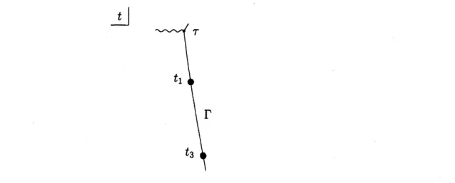
in Figure

1.

$\lrcorner t$

Fig. 1 : Stokes

curve

$\Gamma$ of _{$(NY)_{2}$}

emanating from$\tau=-1.6276-0.0986\sqrt{-1}$

.

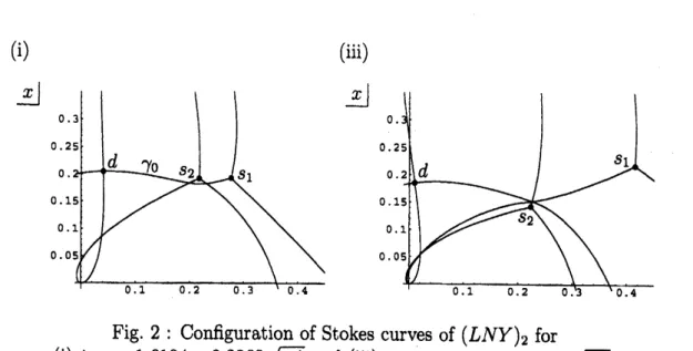
Figure 2 (i) and (iii) indicate the configuration _{of Stokes}

_curves

_of $(LN\mathrm{Y})_{\mathit{2}}$

for $t=t_{1}=-1.6104-0.2268\sqrt{-1}$ _and _{$t=t_{3}=-1.5783-0.4130\sqrt{-1}$}

_on

_the

Stokes

curve

$\Gamma$, respectively. In Figure

2 (i)

a

simple ordinary turning point $s_{1}$ and

a double

ordinary turning point $d$

are

curve

(10)

(i) (iii)

Fig.

2

: Configuration of

Stokes

curves

of $(LNY)_{2}$ for

(i) $t_{1}=-1.6104-0.2268\sqrt{-1}$ _and (iii) $t_{3}=-1.5783-0.4130\sqrt{-1}$

.

consistent with the claim of Proposition 1. (Here, instead of$a_{l}$ and $b_{j}$,

we use

the

symbol $s_{k}$ and $d$respectively to denote a simple turning point and

a

double

one

for

the sake of simplicity.) In Figure 2 (iii), _{however, these}

_two

_turning _points

_are

_no

longer connected by

a

Stokes

curve.

This is an effect of the following

bifurcation

phenomenon ofStokes

curves:

It is readily surmised that

a

simple ordinary turning

point $s_{2}$ should

cross

the Stokes

curve

$\gamma_{0}$ connecting $d$ and $s_{1}$

as

$t$

moves

from $t_{1}$

to $t_{3}$, say at _{$t=t_{2}$}. This actually

occurs.

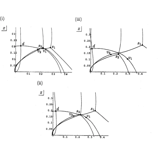
As

a

matter of

fact, if

we

add relevant

virtual turning points and

new

Stokes

curves

to Figure 2,

we

obtain Figure

3

which

indicates the Stokes geometry of $(LNY)_{2}$ for _{$t=t_{j}(j=1,2,3)$}

.

As

_{is visualized} _in

Figure 3 (ii), at $t=t_{2}$ the doubleturning point $d$ isconnected both with

the simple

turningpoint $s_{1}$ andwith

a

virtualturning point

$v_{1}$

.

(Similarly $s_{1}$ is connected both with $d$ and with another virtual turning point

$v_{2}.$) This is a typical

“bifurcation

of

Stokes curves”

discussed

in [AKSST] and [S1]; at $t=t_{2}$ the

relative location

of

an

ordinary

Stokes

curve

emanating

from

$d$ and that of a

new

Stokes

curve

emanating from$v_{2}$

are

interchanged

on

the right of their crossing point and consequently,

when

$t$reaches _{$t=t_{3}$}, the target of the

Stokes

curve

emanatingfrom$d$is switched from

$s_{1}$ to$v_{1}$

.

Thus at$t=t_{3}$ the double turning point$d$is connected with the virtual turning

point $v_{1}$ and simultaneously the simple turning point

$s_{1}$ is connected with $v_{2}$

.

In thisway in

some

portion of theStokes

curve

$\Gamma$ of_{$(N\mathrm{Y})_{2}$}

a

new kind

ofdegeneracyof

the

Stokes

geometryof$(LN\mathrm{Y})_{2}$ is observed;

an

ordinary turning point and

a

virtual

turning point

are

connected by

a Stokes

curve

there.

We also note that,

as

is shown in Figure 3 (i), the two virtual turning points $v_{1}$

and $v_{\mathit{2}}$ are connected by a (new)

Stokes

curve

at

$t=t_{1}$, i.e. in

a

portion of $\Gamma$

near

the turning point $t=\tau$ of $(N\mathrm{Y})_{2}$, in addition to the already-mentioned degeneracy

that $d$ and

$s_{1}$

are

connected by the Stokes

curve

$\gamma_{0}$

.

Bifurcation

of Stokes

curves

is a commonly observed phenomenon for the

(11)

(i) _(iii) $\lrcorner x$

(ii)

Fig.

3: Stokes

geometry of $(LNY)_{2}$ with virtual turning points added.

(Figure (i) is for $t=t_{1},$ $(\mathrm{i}\mathrm{i})$ for $t=t_{2}$ and (iii) for _{$t=t_{3}.$})

$m\geq 3$

.

In Particular, in the

case

_of _{$(LNY)_{2m}$} _{that underlies} _the

_Noumi-Yamada

system $(NY)_{2m}$, as

an

effectof_these_{phenomena degenerate configurations of}_Stokes

curves

of$(LN\mathrm{Y})_{2m}$, i.e.

two

ordinary $\mathrm{a}\mathrm{n}\mathrm{d}/\mathrm{o}\mathrm{r}$ virtual turning pointsbeingconnected

by

a Stokes

curve,

can

be found simultaneously

atseveral placeswhen the parameter $t$ lies

on a Stokes

curve

of$(N\mathrm{Y})_{2m}$,

as

is exemplified by Example 1. This shows

an

important role ofvirtual turning points in _{the theory of isomonodromic}

deforma-tions ofhigher order linear equations or systems of first order linear equations with

size $m\geq 3$; virtual turning points

are

_{indispensable} _{for the} _{complete description} _of

such degeneracy of the Stokes geometry.

4.3 _{Sasaki’s observation for}

_the

_creation

_of

_new

_Stokes

_curves

of

$(N\mathrm{Y})_{2m}$

In his master _{thesis and its successive paper} _(cf. _{[Sl, S2])}

_Sasaki

_{has made}

_an

(12)

$(NY)_{2m}$

.

Virtual turning points of the underlying Lax _pair _{$(LNY)_{2m}$} _play _an

im-portant role also there (in a complicated and somewhat mysterious way). In the

final section of this report

we

discuss

Sasaki’s

observation by using $(NY)_{4}$ and its

underlying Laxpair $(LN\mathrm{Y})_{4}$.

Example 2. $([\mathrm{S}2])$ Let

us

consider the following

Noumi-Yamada

system _{$(NY)_{4}$}:

$(NY)_{4}$ $\{$ $-1du_{0}$ $\eta$ $\overline{dt}$ $=$ $u_{0}(u_{1}-u_{2}+u_{3}-u_{4})+\alpha_{0}$, $-1du_{4}$ $\eta$ $\overline{dt}$ $=$ $u_{4}(u_{0}-u_{1}+u_{2}-u_{3})+\alpha_{4}$

.

Here $\alpha_{0}+\cdot.$

.

$+\alpha_{4}=\eta^{-1}$ and _{$u_{0}+\cdot.$}

.

_{$+u_{4}=t$}

are

satisPed

and

we

take the

following particular value of

_Parameters:

$\alpha_{0}=1-0.35\sqrt{-1},$ $\alpha_{1}=0.45-0.7\sqrt{-1}$,

$\alpha_{2}=-0.5-0.2\sqrt{-1}$ and $\alpha_{3}=-1.05+0.25\sqrt{-1}$

.

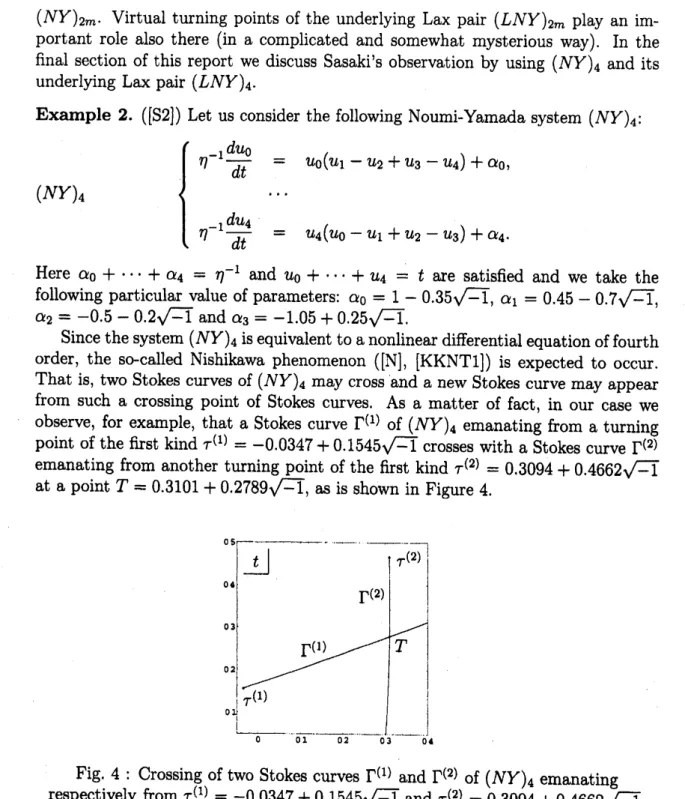
Since

thesystem $(N\mathrm{Y})_{4}$isequivalentto

a

nonlinear

differential

equationof

fourth

order, the so-called Nishikawa phenomenon ([N], [KKNTI]) is expected to

occur.

That is, two Stokes

curves

of $(NY)_{4}$ may

cross

and a new Stokes

curve

may appear

from such a crossing point of

Stokes

curves.

As

a

matter of fact, in

our

case

we

observe, for example, that

a

Stokes

curve

$\Gamma^{(1)}$ of

$(N\mathrm{Y})_{4}$ emanating from

a

turning

point ofthe first kind $\tau^{(1)}=-0.0347+0.1545\sqrt{-1}$

crosses

_with

_a

_Stokes

_curve

$\Gamma^{(2)}$

emanating from another turning point of the first kind $\tau^{(2)}=0.3094+0.4662\sqrt{-1}$

at

a

point $T=0.3101+0.2789\sqrt{-1}$,

as

_is

_shown

_in _{Figure 4.}

Fig. 4 : Crossing oftwo Stokes

curves

$\Gamma^{(1)}$ and $\Gamma^{(2)}$ of

$(NY)_{4}$ emanating

respectively from $\tau^{(1)}=-0.0347+0.1545\sqrt{-1}$_and $\tau^{(\mathit{2})}=0.3094+0.4662\sqrt{-1}$

.

To examineif a

new

Stokes

curve

of$(NY)_{4}$ appears from this crossing_point_$T$_,

we

investigate_{the change of the}_Stokes_geometry_of_(the_first _equation_of)_{the underlying}

Lax pair $(LNY)_{4}$ around the crossing _point. _First _of _all, _the _Stokes

geometry of

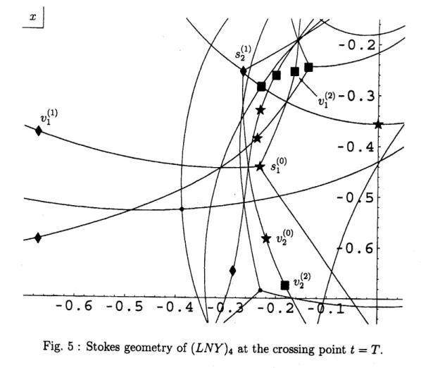
$(LNY)_{4}$ at _$t=T$ is provided in Figure 5.

_Although

_{it is}

_a

_quite

(13)

Fig. 5: Stokes geometry of $(LNY)_{4}$ at the crossing point _$t=T$

.

we can

recognize that

there

exist several tripletsof(ordinary$\mathrm{a}\mathrm{n}\mathrm{d}/\mathrm{o}\mathrm{r}$ virtual) turning

points that

are

connected by

a Stokes

curve

of $(LNY)_{4}$

.

This is actually effected

by the

fact

that $t=T$ is a crossing point of the two Stokes

curves

$\Gamma^{(1)}$ and $\Gamma^{(2)}$ of

$(NY)_{4}$

.

For

example,

as

_$t=T$ _{lies in} $\Gamma^{(1)}$

an

ordinary simple turning point $s_{1}^{(0)}$ is connected with a virtual turning point $v_{1}^{(1)}$ by a

Stokes

curve, and simultaneously $s_{1}^{(0)}$

is connected with _{another virtual} _turning _point $v_{1}^{(\mathit{2})}$ as

$t=T$ lies in $\Gamma^{(2)}$

.

That

is, $\{s_{1}^{(0)}, v_{1}^{(1)}, v_{1}^{(2)}\}$forn

$1\mathrm{S}$ such atriplet of turning points.

Similarly,

a

virtual turning

point $v_{2}^{(0)}$ is connected

both with

an

ordinary simple turning point $s_{\mathit{2}}^{(1\rangle}$ and

with

a

virtual turning point $v_{2}^{(2)}$; $\{v_{2}^{(0)}, s_{2}^{(1)}, v_{2}^{(2)}\}$ gives another triplet.

In Figure

5 we

may

find at least five such triplets of turning points connected by a Stokes

curve.

On

$\Gamma^{(1)}$ (resp., $\Gamma^{(2)}$) a

turningpoint designated by the symbol

₂

(resp., $\blacksquare$) is connected

with

a

turning point designated by $\star$

.

A turning point designated by

$\star$ hinges

two _{degeneracies of the} _Stokes _{geometry of} $(LNY)_{4}$ and it is call$e\mathrm{d}$ a “hinging (or,

shared) turning point” _{in what}

_follows.

_Of

_course,

_{the existence} _{of (not one, but)}

several triplets ofsuch turning points is

an effect

of the

bifurcation

phenomena of

Stokes

curves

discussed

in the precedent _subsection.

(14)

crossing point $t=T$

.

_{To avoid} _{presenting complicated figures,}

_we

_see

_{the change of}

configurations ofStokes

curves

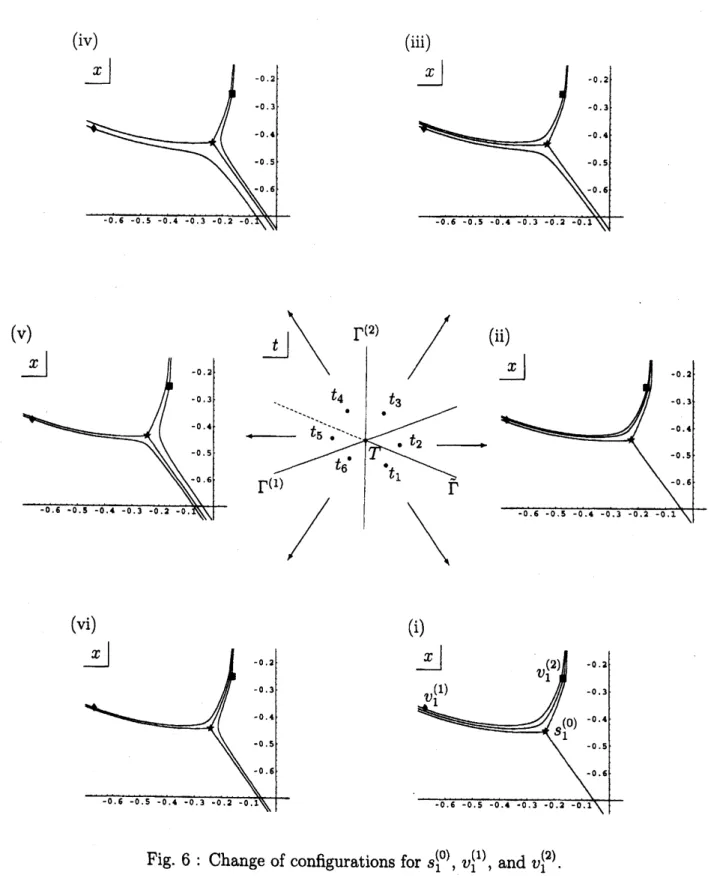
relevant to each triplet ofturning points separately. Let

us

start with a triplet $\{s_{1}^{(0)}, v_{1}^{(1)}, v_{1}^{(2)}\}$

.

Figure 6 indicates the

change of config-urations for this triplet $\{s_{1}^{(0)}, v_{1}^{(1)}, v_{1}^{(2)}\}$

.

As is clearly visualized there, the relative

location of

a

Stokes

curve

passing through $v_{1}^{(1)}$ and that passing through $s_{1}^{(0)}$

are

interchanged both between Figures (ii) and (iii) and between Figures (v) and (vi).

This isdueto the fact that these two turning points$v_{1}^{(1)}$ and $s_{1}^{(0)}$

are

connected by a

Stokes

curve

when the parameter $t$ lies in $\Gamma^{(1)}$

.

Similarly, the

topological

configura-tions

are

different both between Figures (iii) and (iv) and

between

Figures (vi) and

(i) since

on

$\Gamma^{(2)}$ the two turning points $v_{1}^{(2)}$ and $s_{1}^{(0)}$

are

connected

by

a Stokes

curve.

However, in addition to these differences,

we

can

also observe another difference;

the relativelocations of Stokes

curves

passing through$v_{1}^{(1)}$ and $v_{1}^{(2)}$

are

interchanged

between Figures (i) and (ii). This

difference

means

that between the two points

$t_{1}$ and $t_{\mathit{2}}$ there should pass a

new

Stokes

curve

$\tilde{\Gamma}$

of $(NY)_{4}$ where the two virtual

turning points $v_{1}^{(1)}$ and $v_{1}^{(2)}$

are

curve

of

$(LN\mathrm{Y})_{4}$

.

Note that

on

the other side of this

new

Stokes

curve,

that is,

between

the

two

Figures (iv) and

(v)

we

cannot observe

any difference

of topological

configurations; the

new

Stokes

curve

$\tilde{\Gamma}$

of $(NY)_{4}$ is inactive there. The change of configurations

described

_in

Fig-ure

6 is exactly the

same as

that in the

case

of

a

higher order member of the $(P_{J})$

hierarchy ($J=\mathrm{I}$,II-1, II-2) which

we discussed

in [KKNTI]

(see also [N]). Thus we

may conclude that the Nishikawaphenomenon is occurring at this crossing point $T$

of Stokes

curves

of the

Noumi-Yamada

system $(N\mathrm{Y})_{4}$

.

The situation, however, is not so simple

as

in the

cas

$e$ of the $(P_{J})$ hierarchy

($J=\mathrm{I}$, II-1,II-2). In fact, if

we

were

to guess simple-mindedly

the change of config-urations of Stokes

curves

relevant to another triplet $\{v_{2}^{(0)}, s_{2}^{(1)}, v_{\mathit{2}}^{(2)}\}$ in parallel with Figure 6, we should obtain Figure7. In Figure 7we readily findthat the topological

configurations

are

also different

between

Figures (iv) and (v). This does not

seem

consistent with Figure

6.

What is

a

problem? Where does this

inconsistency

come

from?

If

we

trace the change of configurations for the triplet $\{v_{\mathit{2}}^{(0)}, s_{2}^{(1)}, v_{2}^{(2)}\}$

more

pre-cisely and carefully with taking the global structure of the Stokes geometry of

$(LNY)_{4}$ into account, we obtain Figure 8. According _to _{Figure 8,}

_{we can}

_say

the

answer

to the above question is that the virtual turning point $v_{2}^{(2)}$ should

“disap-pear” in the left halfplane of $t$-space (i.e. in the left side

of the Stokes

curve

$\Gamma^{(2)}$ of $(NY)_{4})$ and this disappearance of $v_{2}^{(\mathit{2})}$

recovers

the consistency with Figure 6,

i.e. the change of configurations for the other triplet $\{s_{1}^{(0)}, v_{1}^{(1)}, v_{1}^{(\mathit{2})}\}$

.

As

a

matter of fact, in Figure 8 no difference is observed between the topological configurations ofFigures (iv) and (v) _{since the} _{virtual turning point} $v_{2}^{(2)}$ and

a

new

Stokes

curve

emanating fromit disappear there.

Consequently

Figure

_{8 becomes}

_completely

(15)

$(\mathrm{i}\mathrm{v}\mathrm{l}$ (iii)

(v)

(vi) (il

(16)

(iv) $\lrcorner x$ (iii) $\lrcorner x$ (v) $\lrcorner x$ (vi) (i) $\lrcorner x$ $\lrcorner x$

(17)

(iv) (iiil

(vi

$l\mathrm{v}\mathrm{i})$

(i)

(18)

In [S2] such

a

virtual turning point

as

$v_{2}^{(2)}$ is called a “napping virtual turning point”; it appears only in

a

half plane of $t$-space (“$\mathrm{w}\mathrm{a}\mathrm{k}\mathrm{i}\mathrm{n}\mathrm{g}$ region”, the right side

of $\Gamma^{(2)}$ in the

case

of$v_{2}^{(2)}$), while it disappears in the opposite half plane of t-space (“sleeping region”, the left side of $\Gamma^{(2)}$ in this case). The existence of

a

napping

virtual turning point

saves

us

from the inconsistency mentioned above and

confirms

the appearance of

a

new

Stokes

curve

$\tilde{\Gamma}$

of $(NY)_{4}$ at the crossing point $t=T$

.

Here let

us

briefly explain the

reason

why the changeof the state (i.e. “waking”

or

“sleeping”)

of

$v_{2}^{(\mathit{2})}$

occurs.

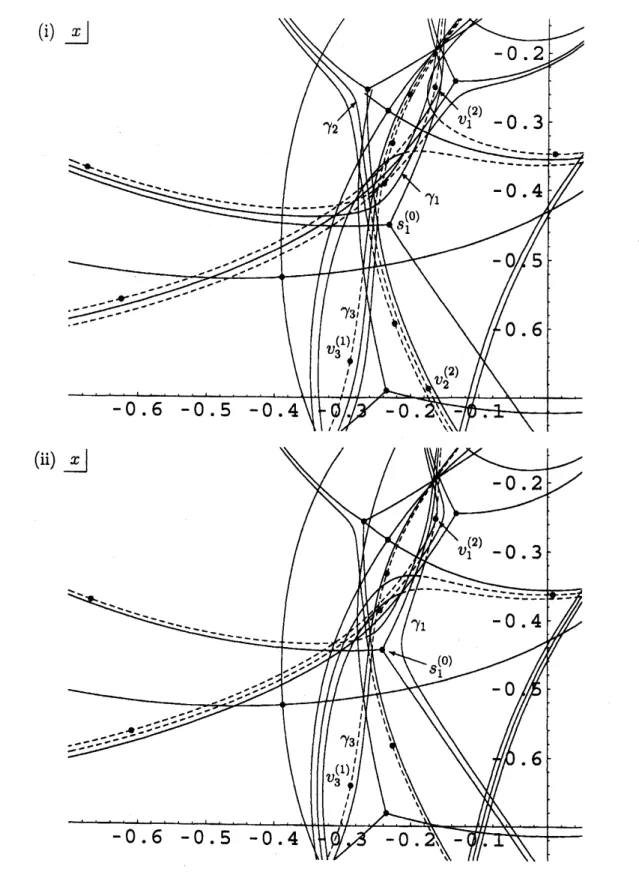
Figure

9

(i) shows the configuration ofallthe relevant

Stokes

curves

at a point (say, $t_{1}$) in the waking region of$v_{2}^{(\mathit{2}\rangle}$

.

Figure 9 (i) tells

us

that

a new

Stokes

curve

$\gamma_{2}$ emanatingfrom thevirtual turning point

$v_{\mathit{2}}^{(2)}$ inquestion

appears in conjunction with thecrossing of

a new

Stokes

curve

$\gamma_{1}$ emanatingfrom a

virtualturning point $v_{1}^{(2)}$ and

a new Stokes curve

$\gamma_{3}$ emanating fromanother virtual

turning point $v_{3}^{(1)}$

.

On

the other hand, the configuration at

a

point (say, _{$t_{11}$}) in the sleeping region of $v_{2}^{(2)}$ becomes

as

is described in Figure

9

(ii). In Figur$e9(\mathrm{i}\mathrm{i})$

the relative location of the

new

Stokes

curve

$\gamma_{1}$ emanating from

$v_{1}^{(2\rangle}$ and that of

a

Stokes

curve

emanatingfrom

an

ordinary turning point$s_{1}^{(0)}$

are

interchanged

so

that

$\gamma_{1}$ goes downward to the right.

As

its consequence $\gamma_{1}$

no

longer

crosses

with $\gamma_{3}$ in

Figure 9 (ii). Hence the

new Stokes

curve

$\gamma_{2}$ and its starting point

$v_{2}^{(2)}$ disappear

there. This is the mechanism that induces the change of the status of the napping

virtual turning point $v_{2}^{(2)}$

.

Such

a

subtle mechanism related to the global structure

ofthe Stokes geometry produces

a

nappingvirtual turning point.

Wefinally note that in the

case

of$\{v_{2}^{(0)}, s_{\mathit{2}}^{(1)}, v_{2}^{(2)}\}$

a

hinging (or, shared) turning point is a virtual turning point $v_{2}^{(0)}$

.

This caused the above apparent inconsistency betweenthe change ofconfigurations

for

$\{v_{2}^{(0)}, s_{2}^{(1)}, v_{2}^{(2)}\}$ and that

for

the

other

triplet $\{s_{1}^{(0)}, v_{1}^{(1)}, v_{1}^{(2)}\}$ whosehinging turning point is

an

ordinaryturning point $s_{1}^{(0)}$

.

In

case

a

hinging (or, shared) turningpointof

a

triplet in questionis

a

virtualturning point,

we believe that

a

napping virtual turning point should be contained in this triplet

to avoid such apparent inconsistency.

In conclusion, at

a

crossing point of two Stokes

curves

of the Noumi-Yamada

system $(NY)_{2m}(m\geq 2)$ we

can

$\exp e\mathrm{c}\mathrm{t}$ the following:

AssumethattwoStokes

curves

$\Gamma^{(1)}$ and$\Gamma^{(2)}$ of_{$(NY)_{2m}$}

cross

at$t=T$

.

In this situation,

as

is discussed in the precedent subsection, for each

Stokes

curve

$\Gamma^{(k)}(k=1,2)$ there should exist several pairs of (ordinary

$\mathrm{a}\mathrm{n}\mathrm{d}/\mathrm{o}\mathrm{r}$ virtual) turning points $\{x_{j}^{(k)}(t),\tilde{x}_{j}^{(k)}(t)\}_{j=1,2},\ldots$ of the underlying

Lax

pair $(LNY)_{2m}$

that

are

connected by

a Stokes

curve

simultaneously.

Then, if every pair $\{x_{j}^{(1)}(t),\tilde{x}_{j}^{(1)}(t)\}$ for $\Gamma^{(1)}$

and the corresponding pair

$\{x_{j}^{(2)}(t),\tilde{x}_{j}^{(2)}(t)\}$ for $\Gamma^{(2)}$ share

one

turning point

and “Lax-adjacency”

(cf. [KKNTI],

see

also Probelm

3

below) holdsthere,

a new

Stokes

curve

of $(N\mathrm{Y})_{2m}$ emanates from the crossing point $t=T$

.

Furthermore, if

a

shared turning point is

a

virtual turning point, a

(19)

Fig. 9 : Configuration ofStokes

curves

of$(LN\mathrm{Y})_{4}$ for (i) $t_{1}$, i.e. in the waking region of$v_{2}^{(2)}$, and (ii)

(20)

In this

manner

virtual turning points of $(LNY)_{\mathit{2}m}$ play

an

important role also for

the creation of new Stokes

curves

of Noumi-Yamada systems $(N\mathrm{Y})_{2m}$.

However, there still remain many things to be studied. In ending this report,

we

list up

some

problems concerning the creation of

new

Stokes

curves

of

Noumi-Yamada systems $(N\mathrm{Y})_{2m}$

.

Problem 1. To study analytic properties (e.g. the connection formulas) for Stokes

phenomena

on

bothordinary and

new

Stokes

curves

of $(NY)_{2m}$

.

This is the most important problem for the global study of solutions of

Noumi-Yamadasystems. To discuss Problem 1

we

need deeper

_{understanding for}

_the

_Stokes

geometryof the underlying

Lax

pair $(LN\mathrm{Y})_{2m}$

discussed

in thisreport.

For

example,

the following points should be clarified.

Problem

2. Oneach Stokes

curve

of $(N\mathrm{Y})_{2m}$

there

exist several pairs

of

(ordinary

$\mathrm{a}\mathrm{n}\mathrm{d}/\mathrm{o}\mathrm{r}$ virtual) turning points of _{$(LN\mathrm{Y})_{\mathit{2}m}$} that

are

connected by

a

Stokes

curve

simultaneously, and at

a

crossing point of two Stokes

curves

of $(NY)_{2m}$ fromwhich

a new

Stokes

curve

starts there exist several triplets of turning points of $(LNY)_{2m}$

connected by

a

Stokes

curve

simultaneously. Then,

are

all triplets ofturning points

equally important for the study of Stokes phenomena

on

the

new Stokes curve,

or

only

a

part of them relevant to Stokesphenomena? If onlyasmall number of triplets

are

concerned with Stokes phenomena, how should

we

choose them?

Problem 3.

The _{“Lax-adjacency”, i.e. the key property}

_that

_determines

_whether

_a

new

Stokes

curve

doesreallyappear

or

not at

a

crossing pointof

two

Stokes

curves

of

a

higher order Painlev\’e equation, isdefined in [KKNTI] for the Painlev\’e_hierarchies

$(P_{J})$ ($J=\mathrm{I}$,II-1, II-2) where the size of the underlying Lax

pair is $2\cross 2$

.

Then,

what is the precise definition of the “Lax-adjacency” for

Noumi-Yamada

systems

$(N\mathrm{Y})_{2m}$?

To

answer

these problems

we

need to develop

more

systematic study ofthe

Stokes

geometry of$(LNY)_{2m}$

.

Recently Honda_hasbeen undertaking _such _{systematization.}

The details ofhis study will be reported in [H].

References

[AKSST] T. Aoki, T. Kawai, S. Sasaki,

A. Shudo

and Y. Takei, Virtual turning

points and

bifurcation

of

Stokes curves

for higher _{order ordinary}

differen-tial equations, J. Phys. A, 38(2005),

3317-3336.

[AKTI] T. Aoki, T. Kawai and Y. Takei, New turning points in the exact

WKB analysis for higher-order ordinary

differential

equations, Analyse

alg\’ebrique des perturbations singuli\‘eres. _{I, Hermann, Paris, 1994, pp.}

(21)

[AKT2] –, WKB analysis of Painlev\’e transcendents with a large

parame-ter. II, Structure of Solutions of Differential Equations, World Scientific, 1996, pp.

1-49.

[BNR] H.L. Berk, W.M. Nevins and K.V. Roberts, New Stokes’ line in WKB

theory, J. Math. Phys., 23(1982),

988-1002.

[H] N. Honda, Toward the complete description of the Stokes geometry, in

preparation.

[KKNTI] T. Kawai, T. Koike, Y. Nishikawa and Y. Takei, On the Stokes geometry

of higher order Painlev\’e equations, Ast\’erisque, Vol. 297, 2004, pp.

117-166.

[KKNT2] –,

On

the complete description ofthe Stokes geometry for the first

Painlev\’e _hierarchy,

_RIMS

_{K\^oky\^uroku,} _Vol. _{1397, 2004,} _pp.

_74-101.

[KT1] _{T. Kawai and} Y. Takei, WKB analysis of Painlev\’e _{transcendents with}

_a

large parameter. I, Adv. Math., 118(1996),

1-33.

[KT2] –, WKB analysis of Painlev\’e transcendents with

a

large

parame-ter. III, Adv. Math., 134(1998), 178-218.

[KT3] –, AlgebraicAnalysis ofSingular Perturbation Theory, Translations

of

Mathematical

Monographs, Vol. 227, Amer. Math. Soc.,

2005.

(Origi-nally published in Japanese by Iwanami, Tokyo in 1998.)

[N] Y. Nishikawa,

Towards

the exact WKB analysis of the $P_{\mathrm{I}\mathrm{I}}$ hierarchy,

sub-mitted.

[NY] M. Noumi andY. Yamada, Higher order Painlev\’e equations of type $A_{l}^{(1)}$,

Funkcial

Ekvac., 41(1998),

483-503.

[S1] S. Sasaki, The _{role of virtual turning points in} _{the deformation of} _higher

order linear ordinarydifferentialequations. I, RIMSK\^oky\^uroku, Vol. 1433,

2005, pp.

27-64.

(In Japanese.)

[S2] –, The role of virtual turning points in the deformation of higher

order linear ordinary

differential

equations. II, ibid., pp.

65-109.

(In

Japanese.)

[T1] Y. Takei, An explicit description of the connection

formula

for the first

Painlev\’eequation, Towardthe Exact WKB Analysis of Differential

Equa-tions, Linear

or

Non-Linear, Kyoto Univ. Press, 2000, pp.

_271-296.

[T2] –, Toward the exact WKB analysis for higher-order Painlev\’e

equa-tions –The

case

of

Noumi-Yamada

systems, Publ. RIMS, Kyoto Univ.,