States with $v_1 = \lambda, v_2 = -\lambda$ and reciprocal equations in the six-vertex model(Solvable Lattice Models 2004 : Recent Progress on Solvable Lattice Models )

cond-mat/0506613

States with

$v_{1}=\lambda,$ $v_{2}=-\lambda$

and

reciprocal

equations

in

the

six-vertex

model

M.J.

Rodr\’iguez-Plazai

Departamento de Fisica Te\’orica$I$, Facultadde Ciencias Fisicas

Universidad Complutense de Madrid,

₂₈₀₄₀

Madrid, Spain

Abstract

The eigenvalues of the transfermatrixin asix-vertexmodel (withperiodic boundary

condi-tions)

can

bewritten in termsof $n$ constants $v_{1},$_$\ldots,$$v_{n}$, the

zeros

ofthefunction $Q(v)$

.

A

peculiarclass of eigenvalues

are

those in which two of the constants $v_{1},$ $v_{2}$

are

equal to $\lambda,$$-\lambda$, with $\Delta=-\cosh$A and $\Delta$ related to the Boltzmann weights of thesix-vertexmodelbythe

usualcombination $\Delta=(a^{2}+b^{2}-c^{2})/2ab$

.

Theeigenvectorsassociated to these eigenvalues

are Bethe states(although theyseemnot). Wecountthe number of such states (eigenvectors)

for $n=2,3,4,5$ when $N$, thecolumnsina rowofa squarelattice,is arbitrary. The number

obtained isindependent of the value of $\Delta$, but dependson _$N$

.

We give the explicit

expres-sion of the eigenvalues in terms of $a,$$b,$ $c$ (when possible)orin termsoftherootsofacertain

reciprocal polynomial, beingverysimpleto reproduce numerically these special eigenvalues

for arbitrary $N$ in the blocks $n$ considered. For real $a,$$b,c$ such eigenvalues are real.

$PACS$_numbers: 05.50.$+q7\mathit{5}.\mathit{1}\theta.Hk$

Keywords: Statistical mechanics; six-vertex model;

_transfer

$mat’\dot{\mathrm{w}}_{i}$ Bethe ansatz; $Q(v)$ function; $|\mathfrak{r}ci\mathrm{p}\mathrm{r}ocal$

polynomial

1 Theproblem

Sometime

ago

the author ofthis note read in thepaper Completeness

_of

the Bethe Ansatz

_for

the Six

and Eight-

Vertex

Models by R.J Baxter [1, Sect. 4] the following sentenceconcerning certain

proper

states of the transfer matrixin the six-vertex model at zero-field:

The other problem that we encountered first occurs for $N=4$ and $n=2$, thenfor even $N$ and $2\leq n\leq N-2$

.

_{It is referred to byBethe himself and has been considered by others}

since2.

_{For some} eigenvalueswith momentum $\pm 1$, 3i.e. _{$k_{1}+\cdots+k_{n}=0$} or $\pi_{)}$wefound that

$Q(v)= \prod_{j=1}^{n}\sinh[(v-v_{j})/2]$ hadapairofzeros $v_{1},$ $v_{2}$ such that $v_{1}=\lambda,$$v_{2}=-\lambda$

.

1E–mail: $\mathrm{m}\mathrm{j}\mathrm{r}\mathrm{p}\mathrm{l}u\mathrm{a}\emptyset \mathrm{f}\mathrm{l}\mathrm{s}.\mathrm{u}\mathrm{c}\mathrm{m}.\infty$

$2$

[$2$, aftereq. (23)],$[3],$ $[4],$ $[5]$

The lines continued lateras follows:

For $N=4$ therewasjustonesucheigenvalue $\Lambda$, in the $n=2$ central block. For $N=6$ therewas onein

the $n=2$ block, two in the $n=3$ block, andonein the $n=4$ block. For $N=8$ there were 1, 2, 5, 2, 1 in the $n=2,3,4,5,\mathit{6}$ blocks,respectively. Thissuggests (tentatively)that theCatalannumbersmaycount such

eigenvalues.4

The momentawere $-1$ exceptfor a single eigenvalue with momentum +1 in each block with $3\leq n\leq N-3$

.

If the author had understood properly the eigenvectors associated to such eigenvalues and how to

obtainthemfrom Betheansatz,probablywould have notdetained

so

long when reading these sentences.

But that

was

not the

case: we were

calculating atthat time the free.energy per site ofavertex model

whose ground state

was a

stateofthistype, andthevalue ofthefree-energythat

we were

deriving

was

once

andagain the incorrect

one.

Wedecidedin

consequence

to putaside thefree-energyproblemfor

a

time and studyinstead these statesin the six-vertex model. We ignore the correct

name

that

we

shall

use

for them. In the literature they have received the

name

ofsingularBethe states

or

singularities

of the Bethe solutions [3, 4, 6], and also non-Bethe eigenvectors [7]. We might even remember

some

references inwhichthey

are

alluded

as

improperstates. Since they need

a

name

and nootherstates

are

considered inthispaperwe will refer tothem

as

boundpairs merely.

Thisnotecommunicates

some

results of thestudyand

answers

theinterrogation suggested inBaxter’s

paper: Are Catalan numbers counting the boundpair states

_of

a square six-vertex model with periodic

boundary $conditions^{Q}$

2 The $\mathrm{m}o$del

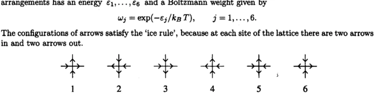
Themodel to beconsidered is a six-vertex model in a square lattice $[8, 9]$

.

In this model to eachsite

of the latticeis associated

one

of thesixarrangementsof

arrows

shownin figure 1, where each of these

arrangementshas an

energy

$\epsilon_{1},$$\ldots,\epsilon_{6}$ and

a

Boltzmannweight givenby

$\omega_{j}=\exp(-\epsilon_{j}/k_{B}T)$, $j=1,$$\ldots$, 6.

Theconfigurationsof

arrows

satisfythe ‘icerule’,becauseateachsiteofthe latticethere

are

two

arrows

inand two

arrows

out.

$\not\simeq$ $\prec\#$ $\not\simeq$

$1$

2

3

$\not\simeq$ $arrow*\iota$ $\not\simeq$

$4$

5

6

Figure 1. Thesixconfigurationsallowed atavertex. At each site of the lattice there aretwoarrows inand two arrowsout.

Thisis knownasthe ‘ice-rule’.

Suppose that the lattice has dimensions $M\mathrm{x}N$, that is $N$ sites horizontally and $M$ vertically,

with theimpositionofperiodic boundary conditions in both directions. Thestate of

an

arbitrary

row

of $N$ vertical edges is then specified by the configuration ofup and down

arrows on

the edge. Let

$\sigma=(\sigma_{1}, \ldots, \sigma_{N})$ denote thestate ($\sigma_{j}=+1$ for

an

up

arrow

atvertex $j,$ $\sigma_{j}=-1$ fora downarrow).

If $\sigma$ is the stateofa

row

and $\sigma’$ the stateof the rowbellow, thetwo adjacentstates

are

coupled by

the transfer matrix $T_{\sigma\sigma’}$, whose entries

are

given by

a

traceof 2$\mathrm{x}2$ matrices

$T_{\sigma\sigma’}=\mathrm{t}\mathrm{r}\mathrm{a}\mathrm{c}\mathrm{e}R_{\sigma_{1}\sigma_{1}’}R_{\sigma_{2}\sigma_{2}’}\cdots R_{\sigma_{N}\sigma_{N}’}$ , (2.1)

where

$R_{++}=,$

$R_{+-=}$ ,

$R_{-+}=$

,

$R_{--}=$

.

A consequenceofthe (ice_{rule’ together with thehorizontalperiodicityof thelatticeisthatthe number}

$n$ ofdown (or up) arrowsina rowis

a

conserved quantity fromrowto row,and $T$,a $2^{N}\cross 2^{N}$ matrix,

breaksup into $N+1$ diagonalblocks withone block for each value $n=0,1,$$\ldots$,$N$

.

Thedimension of

block $n$ is

of the lattice $Z=\mathrm{t}\mathrm{r}\mathrm{a}\mathrm{c}\mathrm{e}T^{M}$, and this has implied the diagozalization of matrix $T$

.

In the

case

ofa

zero electrical field (the

case

treated here)where

$a=\omega_{1}=\omega_{2}$, $b=\omega_{3}=\omega_{4}$, $c=\omega_{5}=\omega_{6}$, (2.2)

the eigenvalues A of the transfer matrix

are

known tobe [9]

$\Lambda(v)=(-1)^{n}\frac{\phi(\lambda-v)Q(v+2\lambda)+\phi(\lambda+v\rangle Q(v-2\lambda)}{q(v)}$, (2.3)

wherefunctions $\phi(v),$ $Q(v)$

are

$\phi(v)=\rho^{N}\sinh^{N}(v/2)$ (2.4)

$Q(v)= \prod_{j=1}^{n}\sinh[(v-v_{j})/2]$, (2.5)

and $\rho,$ $\lambda,$ $v$

are

defined

so

that

$a= \rho\sinh\frac{1}{2}(\lambda-v)$, $b= \rho\sinh\frac{1}{2}(\lambda+v)$, $c=\rho\sinh\lambda$

.

(2.6)

To write the eigenvalues (2.3) we have to locate $v_{1},$$\ldots,$$v_{n}$ for these eigenvalues. There

are

many

solutions, corresponding to thedifferenteigenvalues.

3 Catalan numbers

or

not

Do Catalan numbers count the bound pairstates

of

a

square six-vertexmodel wath periodic boundary

conditions$Q$The answer

is $no$

.

Aswascommunicated in ref. [1], it is true that for $N=4$ there isonebound pairin the $n=2$ central

block,that for $N=\mathit{6}$ thereare 1,2, 1 in the $n=2,3,4$ blocks, respectively, and that for $N=8$ there

are

1,2,5, 2,1 inthe $n=2,3,4,5,6$ blocks. However, if thecountingstarted inthepreviousreference

hadcontinued it would havefoundthat there

are

1, 2, 6,10 in $n=2,3,4,5^{5}$_for $N=10$, and 1, 2, 7,12

in $n=2,3,4,5$ for $N=12$

.

In fact

our calculations

hereshow thatfor general

even

$N$ the number

isexactly 1, 2,$N/2+1,$$N$ inthe blocks $n=2,3,4,5$

.

The numbers of statesfor $n=6$ and beyond

wont be studied inthis paper.

4 Bound pairs and Bethe Ansatz

To obtain the eigenfunctions of the transfer matrix

one

can

either diagonalize exactly the matrix

(impossible when the size is not reasonable)

or

use the Bethe ansatz, the trial form that Bethe

used for diagonalizing the quantum-mechanical Hamiltonial ofthe one-dimensionalHeisenberg model

[2]. The ansatz suggests that the eigenstate of $T(v)$, $T(v)|\psi\rangle=\Lambda(v)|\psi\rangle$,

can

be written

as

$| \psi\rangle=\sum_{x_{1}<\ldots<x_{*}},f(x_{1}, \ldots, x_{n})|x_{1},$$\ldots,x_{n}\rangle$ ,where thecoefficients $f(x_{1}, \ldots,x_{n})$

are

$f(x_{1}, \ldots,x_{n})=\sum_{P}A_{\mathrm{p}_{1},\ldots,p_{n}}e^{1k_{P1}x_{1}}\cdots e^{1k_{\mathrm{p}n}x_{\mathrm{n}}}$

.

(4.1)

5Weomittomentiontheblocks $n=N/2+1$ to $N-2$ sincethe numberof thesestatesis thesame asinthe blods

The numbers $x_{1},$$\ldots$,$x_{n}$ indicate thepositionsof $n$ down

arrows on

the lower vertical edges of

a

row

of the lattice, and

are

ordered

so

that $1\leq x_{1}<x_{2}<\ldots x_{n}\leq N$

.

We have experienced that the

coefficients $A_{\mathrm{p}_{1},\ldots,p_{\iota}}$, suitable to construct bound

pairs6

aregivenby

$A_{\mathrm{p}_{1},\ldots,\mathrm{p}_{l}},= \epsilon_{P}/C\prod_{1\leq\dot{\iota}<j\leq n}s_{\mathrm{p}_{\mathrm{j}},p:}$ , (4.2)

where $\epsilon_{P}=\pm 1$ isthesignofthepermutation $\{p_{1}, \ldots,p_{n}\}$ of $\{1, \ldots, n\}$ and $C$ is

a

non-zero

constant

to be

fixed

laterinthe most convenient

manner

(usually normalization). The vertex model defined by

activities $a,$$b,$ $c$ sothat

$\Delta=\frac{a^{2}+b^{2}-c^{2}}{2ab}$ (4.3)

enters in $s_{1j}$ ,

defined

as

$s:j=1-2\Delta e^{1k_{j}}+e^{1(k_{\mathrm{t}}+k_{j})}$

.

(4.4)

To writethe eigenstates isonly

necessary

then to know the factors $e^{ik_{1}},$

$\ldots,$

$e^{:k_{n}}$ that appear in (4.1)

and (4.4). These factors

are

the solutions of theequations

$e^{iNk_{p_{1}}}A_{\mathrm{p}_{2\prime}p_{n},p_{1}},\ldots=A_{\mathrm{P}1p},\ldots,,.$ ,

(4.5)

that impose the periodic boundary conditions

on

the problem making that $f(x_{1},x_{2}, \ldots,x_{N})=$ $f(x_{2}, \ldots , x_{N},x_{1}+N)$ what identifies the $N+1$ and 1 vertices. To be (4.5) consistent equations

among

themselves, it is

necessary

that

$e^{iN(k_{1}+\cdots+k_{n})}=1$

.

_(4.6)

Equations (4.1), (4.2), (4.4), (4.5) and (4.6),

are

_sufficient

equationsto writeboundpair eigenfunctions,

andwhenneeded

we

willreferto themas “the Betheansatz equationsfor boundpairs”. However, and

this is not lessimportant, it is alsonecessary

a

correctnormalization of the eigenfunction. Without it,

thestatecannot beobtained. Wehavelearned thecorrectnormalization in ref. [1, Sect.4],and show

an

example later for $N=\mathit{6}$ and $n=3$

.

Equations (8.2), (8.3) and (8.2), (8.3), (8.6)

are

deducedtaking

into account such normalization.

It isimportanttowrite,before finishing, therelation between $k_{1}\ldots,$$k_{n}$ and $v_{1},$_$\ldots,$$v_{n}$ in (2.5) (or better between $e^{:k_{\dot{f}}}$ and $e^{v_{j}}$ )

$e^{:k_{\mathrm{j}}}= \frac{e^{\lambda}-e^{v;}}{e^{\lambda+v_{\mathrm{j}}}-1}$

,

(4.7)

as

mentioned in many papers. This relationpermitsto

move

from theeigenvalue (2.3)tothe eigenvector

(4.1)ofthe transfer matrix when

we

precise it.

5 A change of variables

Before describing any eigenvalue

we

make

a

useful change of variables concerning $v$ and $\lambda$ in (2.6).

The changeis convenientfor those(the author inthisspecificproblem

among

them)whoprefer to work

withpolynomialsrather thanwith hyperbolic functions

as

in(2.5). Define the variables

$z=e^{-v}$, $y=e^{-\lambda}$ (5.1)

6Becausethey give thesameresultthat whenthetransfermatrixis directly diagonalized. When the size of the matrix

instead of $v$ and $\lambda$, then (2.5) is

essentially7

the polynomial in

$z$ and $1/z$ given by

$Q(z)= \frac{1}{z^{n/2}}\prod_{\mathrm{j}\approx 1}^{n}(z-z_{j})$, (5.2)

with $z_{j}=e^{-v_{j}},$ $j=1\ldots,$$n$

.

Tobecorrect

we

should havedefined anothersymbolfor (5.2), $\tilde{Q}(z)$ for

instance, however

we

will

use

the

same

letterwith the understandingthat $Q(v)$ stands for (2.4) and

$Q(z)$ for (5.2). In terms of these variables and togetherwith definitions _(2.4) and _(2.5), relation _(2.3)

becomes

$(2/ \rho)^{N}\Lambda(v)Q(z)=\frac{(-1)^{n}}{(zy)^{N/2}}[(z-y)^{N}Q(zy^{2})+(1-zy)^{N}Q(z/y^{2})]$, (5.3)

where multiplicative constant factors in $Q$ cancel out of the calculations. To operate in

a

computerwe

prefer toworkwith this relation

more

than with (2.3).

6 $\mathrm{n}=2$

Thisis

the

simplest

case

to study because the transfer matrix

of

$N$ edges (with $N$ even)hasonly

one

bound pair state in thisblockfor arbitrary $\Delta$ defined in (4.3). Since boundpairs

are

characterized by

$v_{1}=\lambda,$ $v_{2}=-\lambda$

as

mentioned inSec. 1, function (5.2) factorizes

as

$Q(z)=(zy-1)(z-y)/z$

, (6.1)

the zerosof $Q(z)$ being $z_{1}=y$ and $z_{2}=1/y$

.

Introducedthis functionin (5.3) and noting that the

r.h.s. is exactly divided by $Q(z)$ in thel.h.s,the quotient affords the

eigenvalue8

$\Lambda(v)=a^{2}b^{2}(a^{N-4}+b^{N-4})-c^{2}(a^{N-2}+b^{N-2})$, $N\geq 4$, _$n=2$, (6.2)

thatisvalidforgeneric $N$

even.

It

can

becheckednumericallythat(6.2) is alwaysaneigenvalue of the

transfer matrix forall values of $a,$$b,$ $c$ real

or complex,9

and since the block $n=2$ isamongtheblocks

of smallest dimensions, it

can

be done

even

for $N$ not too small. The eigenvector associated to (6.2)

was knowntoBethe himself [2, also after eq. (23)] and is proportional to

$| \psi\rangle=\sum_{l=1}^{N}(-1)^{l}|l,$$l+1\rangle$, (6.3)

afterappropriatenormalization. Wedonot reproduce here this eigenvectorwiththeBethe ansatz (the

examplethat

we

reproduce is for $N=6,$ $n=3$ later), but want to comment about $e^{:k_{1}}$ and $e^{:k_{2}}$

.

Theproductof these two factorsisfor theeigenfunction (6.3) equalto $-1$, since from (4.1)derivesthe

relation

$f(x_{1}+1,x_{2}+1)=e^{i(k_{1}+k_{2})}f(x_{1},x_{2})$, _with $N+1\equiv 1$, (6.4)

which is simply

a

consequenceofthe translation invarianceofthe transfer matrix(2.1). But also $v_{1}=\lambda$

in (4.7) fixes $e^{:k_{1}}=0$, what obliges to set

$e^{ik_{1}}=-e^{-ik_{2}}=0$_{, (6.5)}

7Essentiallymeans up tomultiplicativeconstants that do not depend on $z$ (theymay dependon $y$ because $y$ is

regarded as aconstant: after all $y$ is fixedby thevalue that we choose for $\Delta$, andviceversa). Theconstants arenot

relevantbecause do not change the value of $\Lambda(v)$, ascommented afterequation (5.3)

$\epsilon\Lambda(v)$ in(5.3)is obtained in terms of

$\iota$ and $y$,ofcourse. We have reexpressed theresultin terms of a,$b,$$c$ to write

(6.2)

$\mathfrak{g}_{a,b,c}$, the Boltzmann weights(2.2) of thevertexmodel,arereal andpositive,but when diagonalization ofamatrix

as was donein [1]. Thishappens for all bound pairs thatwe haveobtained no matter the values of $N$

and $n$: it is simply a

fact

thatfor these states in this model

$e^{i(k_{1}+k_{2})}=-1$

.

(6.6)

Thiscondiction, together with the two identities in (6.5) mark how towork appropiately with bound

pairs.

7 $\mathrm{n}=3$

The trial function (5.2) is

now

of theform

$Q(z)=(zy-1)(z-y)(z-A)/z^{3/2}$ , (7.1)

with $A$ a constant (numerical

or

depending

on

_$y$) to bedetermined. Substituting (7.1) in (5.3), the

r.h.s. of this equation is exactly divided by $Q(z)$ in the l.h.s. if and only if $A=0,$$-1,1$

or

$A$ is

thesolution of

a

certain polynomial whose coefficientsdepend only

on

$\Delta$

.

The root $A=0$ is not

an

admissible solution because (7.1)has not therequired expansion (5.2);

on

the contrary, roots $A=-1,1$

yield admissible functions $Q(z)$ because the associated A(v) by (5.3) are always in the spectrum of

the transfermatrix, as wehaveverifiedin

numerous

experiments. Forexample,the numbers

$\Lambda_{+}\equiv 2a^{3}b^{3}-abc^{2}(a^{2}+ab+b^{2})+c^{4}(a^{2}-ab+b^{2})$, _(7.2) $\Lambda_{-}\equiv 2a^{3}b^{3}-abc^{2}(a^{2}-ab+b^{2})-c^{4}(a^{2}+ab+b^{2})$, (7.3)

areeigenvalues of the $N=6$ transfermatrix for arbitrary values of $a,$$b,$ $c$

.

The first is for $A=-1$,

thesecond for $A=1$

.

We present

some

ofthesenumericaltests inTable 1. Regarding the situation in

which $A$ isthe solutionofacertain polynonial, when $N=6$ such polynomial is

$A^{4}+(8\Delta^{3}-4\Delta)A^{3}+(20\Delta^{2}-14)A^{2}+(8\Delta^{3}-4\Delta)A+1=0$, (7.4)

butithastode discarded because

none

of thefourroots of (7.4) is linked to

an

eigenvalue of the transfer

matrix for arbitrary $\Delta$ (it

can

be checked also with Table 1). There are only two $Q’ \mathrm{s}$ (that is, two

boundpairs intheblock) andtwoeigenvalues.

Table1. In vertical areshownthe 20 eigenvaluesof thetransfer matrix block $N=6,$ $n=3$ fordifferent values of $a,$ $b,$$c$.

The eigenvalues areobtained bynumericaldiagonalization ofthematrix in (2.1), andeachresultapproximatedtothenumber arrayedin thetablewiththe rule of 5. In all theexampleswe havefixed $z,$ $y,$$\rho$, and $a,$$b,$$c$ arederived fromthem through

(2.6). The valuesmarkedwith $+$ and –coincide,nomatter thenumber ofdigitsof accuracy demanded in the computation,

withthetheoretical values (7.2), (7.3) obtained in thispapersolving (5.3). In the third columnit is necessaryto multiply by

$10^{6}$ toobtain the correct eigenvalue. Noticethatwhen _{$\Delta=-1/2$} the bound pair(7.9)isdegenerated and thetransfermatrix

has another linearly independentproperstate with thesameeigenvalue $a^{6}+b^{6}$ . This degeneration happensforatl valuesof $a,$$b,$$c$ and not onlyfor theparticularvalue listed here.

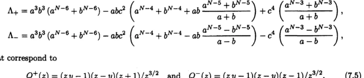
The situation isthe

same

for arbitrary $N$

even:

there

are

onlytwo bound pairs in the blockand

the generalization of(7.2) and (7.3) is

$\Lambda_{+}=a^{3}b^{3}(a^{N-6}+b^{N-6})-abc^{2}(a^{N-4}+b^{N-4}+ab\frac{a^{N-5}+b^{N-5}}{a+b})+c^{4}(\frac{a^{N-3}+b^{N-3}}{a+b})$

,

$\Lambda_{-}=a^{3}b^{3}(a^{N-6}+b^{N-6})-abc^{2}(a^{N-4}+b^{N-4}-ab\frac{a^{N-5}b^{N-b}}{ab}=)-c^{4}(\frac{a^{N-3}b^{N-3}}{ab}=)$ ,

that correspondto

$Q^{+}(z)=(zy-1)(z-y)(z+1)/z^{3/2}$ _and $Q^{-}(z)=(zy-1)(z-y)(z-1)/z^{3/2}$, (7.5)

respectively. The quotients written in $\Lambda_{\pm}$ above

are

$\mathrm{f}\mathrm{i}\mathrm{c}\mathrm{t}\mathrm{i}\mathrm{t}\mathrm{i}\mathrm{o}\mathrm{u}\mathrm{s}^{1}$because the divisions

can

beperformed

exactly giving asresult polynomials in $a,$$b,$ $c$ with nodenominators.

Each eigenvectorof thetransfer matrix has associatedagiven $Q(z)$,

we

now calculate as anexample

the eigenvector associated to $Q^{+}$ in (7.5) for $N=6$ usingBethe

ansatz.11

For such state the product

$e^{i(k_{1}+k_{2}+k_{3})}=1$_{, (7.6)}

that

can

bejustifiedin several

manners:

one, ifthe eigenvalue is known, (7.2) in

this

case, it is enough

to set $b=0,$ $a=c$ in the eigenvalue. The coefficient of $c^{N}$ is precisely $e^{\mathrm{t}(k_{1}+\cdots+k_{*})}$’ [9];

or

two,

evaluating $(-1)^{n}Q(zy^{2})/Q(z)$ at_{the point $z=1/y[1]$}

.

This gives also such product. Sincethe third

zero ofthe function $Q^{+}$ is at _{$z_{3}=-1$}, relation (4.7) indicates that $e^{1k_{3}}=-1$, that substituted in

(7.6) gives the product $e^{:(k_{1}+k_{2})}=-1$, something that seems_to be sharedby all boundpairs ofthe

model

as we

remarkedin (6.6). For

our

pair holds again (6.5) what makes that the factor $s_{21}$ vanishes

according to (4.4). To obtain the correct boundpairstatethe rule$\mathrm{i}\mathrm{s}^{12}$: calculate the

$s_{1j}$ that donot

vanish (in the present case there

are

five ofthem) with (4.4), keeping onlythe dominant term

as

$e^{:k_{1}}$

goes to zero, andcalculate $s_{21}$ with(4.5). In thismanner,insteadofwritting $‘ s_{21}=0$

’_{in theformulae,}

$s_{21}$ takesthe expressionthatvanishes most rapidly as $e^{:k_{1}}$ goes to

zero.

Thisexpression is

$s_{21}=2\Delta(1+2\Delta)e^{i(N-1)k_{1}}$

,

(7.7)

while

$s_{12}=2\Delta e^{-ik_{1}}$

,

_{$s_{13}=1+2\Delta$}, _{$s_{31}=1$},

$s_{23}=e^{-1k_{1}}$, $s_{32}=(1+2\Delta)e^{-ik_{1}}$

.

(7.8)

Notethat theamplitudesobtained with (4.2) afterthesubstitution of(7.7)and (7.8) do satisfy exactly

equations (4.5),

as

expected. Take

now

$N=6$

.

Inserting the values (4.2) into (4.1)

we

find that for

$1_{\mathrm{I}.\mathrm{e}}.$, introducedby the author tomake the

exPraesions comPact

1iWeinsistonthewords Bethe ansatzbecausesomeauthorsrefer to bound pair statesasnon-Bethestates,and they

areBethestates

example, $f(1,2,3)=-2\Delta(1+2\Delta)^{2}/C$ _and $f(1,2,4)=2\Delta(1+2\Delta)e^{-ik_{1}}/C$

.

_{In the}

_case

_$N=6$

two

more

components

are necessary

to write theeigenvector, namely

$f(1,2,5)=-2\Delta(1+2\Delta)e^{-ik_{1}}/C$_{, $f(1,3,5)=-\mathit{6}\Delta(1+2\Delta)/C$,}

sincethe remaining componentsare deducedfrom thesefour with thegeneralization of property (6.4)to

the

case

$n=3$

.

Clearly $f(1,2,4),$ $f(1,2,5)$

are

_{the elements that grow most} rapidly

as

$e^{ik_{1}}$

vanishes

and the sensible choice here is to take $C$ so that $f(1,2,4)=1$

.

The result is the right eigenvector

associatedto $Q^{+}$ in $(7.5)^{13}$

$|\psi\rangle=|1,2,4\rangle+|2,3,5\rangle+|3,4,6\rangle+|1,4,5\rangle+|2,5,6\rangle+|1,3,6\rangle$

$-|1,2,5\rangle-|2,3,\mathit{6}\rangle-|1,3,4\rangle-|2,4,5\rangle-|3,5,6\rangle-|1,4,6\rangle$, (7.9)

whichcoincides with thevectorfound in [3,

eq.

(22)] using different methods.

8 $\mathrm{n}=4$ and $\mathrm{n}=5$

Thereis

no

problem inrepeatingthe

same

steps

as

in $n=3$ todeducethe number ofboundpairswhen

$n=4$

or

$n=5$

.

In fact introducing

$Q(z)=(zy-1)(z-y)(z^{2}+Az+B)/z^{2}$ _(8.1)

into (5.3), it ispossible to find constants $A$ and $B$

so

that thefunction A(v) is

an

eigenvalue ofthe

transfer matrixblock $n=4$ forarbitrary $a,$$b,$ $c$ activities. However,

we

follow

a

different method in

thissectionwiththeintentionof obtainingabetter trialfunction $Q$ notasgeneralasin(8.1): wesolve

directly Bethe ansatz equations (4.5)

instead14.

Theequations are alreadysolved for $e_{1}$ and $e_{2}$ (for

brevitywe will

use

from

now

the notation $e_{1}$ to denote the number $e:k_{1},$ $e_{2}$ to denote $e^{k_{2}}$, and

so

on), since

we

know that $e_{1}=0,$ $e_{2}=-1/e_{1}$, with the product $e_{1}e_{2}$ equal to $-1$

as

a characteristic

ofboundpairs. Itremainsto solve for $e_{3},$ $e_{4}$ inthe

case

$n=4$, and for $e_{3},$$e_{4},e_{6}$ inthe

case

of $n=5$

.

And

when resolvingthe

same

care

about $s_{1j}$ has to betaken that

when

the eigenfunction (7.9)

was

constructedin the previoussection: $s_{21}$ that vanisheshas to be evaluatedwith (4.5), taking then the

expressionthatvanishes most rapidlyas $e_{1}$ goes to zero, and the remaining $s_{1j}$ with (4.4). Withthese

remarks takeninto consideration theequationsto solve are

$e_{3}^{N-1}=-( \frac{1-2\Delta e_{3}}{e_{3}-2\Delta})(=\frac{12\Delta e_{3}+e_{3}e_{4}}{12\Delta e_{4}+e_{3}e_{4}})$

,

(8.2)

$e_{4}^{N-1}=-( \frac{1-2\Delta e_{4}}{e_{4}-2\Delta})(=\frac{12\Delta e_{4}+e_{3}e_{4}}{12\Delta e_{3}+e_{3}e_{4}})$, $N\geq 8$, (8.3)

inthe block $n=4$, and

$e_{3}^{N-1}=( \frac{1-2\Delta e_{3}}{e_{3}-2\Delta})(=\frac{12\Delta e_{3}+e_{3}e_{4}}{12\Delta e_{4}+e_{3}e_{4}})(=\frac{12\Delta e_{3}+e_{3}e_{6}}{12\Delta e_{5}+e_{3}e_{6}})$, (8.4) $e_{4}^{N-1}=( \frac{1-2\Delta e_{4}}{e_{4}-2\Delta})(=\frac{12\Delta e_{4}+e_{3}e_{4}}{12\Delta e_{3}+e_{3}e_{4}})(=\frac{12\Delta e_{4}+e_{4}e_{5}}{12\Delta e_{5}+e_{4}e_{6}})$, $N\geq 10$ (8.5) $e_{5}^{N-1}=( \frac{1-2\Delta e_{5}}{e_{5}-2\Delta})(=\frac{12\Delta e_{6}+\mathrm{e}_{3}e_{6}}{12\Delta e_{3}+e_{3}e_{5}})(=\frac{12\Delta e_{5}+e_{4}e_{5}}{12\Delta e_{4}+e_{4}e_{6}})$, (8.6)

$\underline{\mathrm{w}\mathrm{h}\mathrm{e}\mathrm{n}n=5.}$Remember that $\Delta \mathrm{i}\S$givenby (4.3) and $N$ is

an

even

number.

i3Fbrgeneral $N$ theeigenvectoris $|\psi\rangle$ $= \sum_{l\approx 1}^{N}(|l,l+1, l+3\rangle-|l,l+2, l+3\rangle)$

.

The state thataccompaniesto $Q^{-}$

is $|\psi\rangle$ $= \sum_{l=1}^{N}(-1)^{l}(|1,l+1,[+3\rangle+|l,l+2,[+3\rangle)$

.

Ithaseomesimilary with(6.3)but intheblock $n=3$

14Once $\epsilon:k_{\theta},$

$\ldots$,

Consider the equations relative to $n=5$ for a moment. Notice that if $(e_{3}, e_{4}, e_{5})$ is a solution ofequations $(8.4)-(8.6)$ _for given $N$ and $\Delta^{15}$, also $(e_{4}, e_{3}, e_{5})$, the interchange of $e_{3}$ with $e_{4}$, is a

solution; and also it is $(e_{3}, e_{5}, e_{4})$

.

Equations $(8.4)-(8.6)$ do not distinghish

a

solution from any of

its permutations. It is for this reason that two solutions

are

considered the

same

if coincide up to

permutations.

There is another relevant property of the equations: if $(e_{3}, e_{4}, e_{5})$ is

a

solution, $( \frac{1}{e_{8}},$$\frac{1}{e_{4}},$$\frac{1}{e_{5}})$ is

also

a

solution for the

same

$N$ and $\Delta$

.

Thisfeature brings considerableinsight into the resolutionof

$(8.4)-(8.6)$

.

For _{example, if} $e_{3}$ is in the solution

so

does $1/e_{3}$,

as

this property establishes, therefore

$1/e_{3}$ is

one

of

the

numbers in $(e_{3}, e_{4}, e_{5})$

.

Ifit is equal toitsinverse, $e_{3}$ is

1 or

$-1$ ,

but

ifnot, the

inverse of $e_{3}$ has to be say, $e_{4}$, andthus $e_{3}e_{4}=1$. The argument is repeatedwith $e_{4}$ to conclude

that $e_{4}$ is 1

or

$-1$ ortheinverseof$e_{3}$

.

Finally, it istheturn of $e_{5}$,that

can

be only $\pm 1$ and notthe

inverse of any other number becausethere

are no more

left numbers to bepaired with.

In

conclusion:

$(e_{3}, e_{4}, e_{5})$ are (1, 1,1), $(-1, -1, -1)$ or _{$(e_{3}, e_{4}, \pm 1)$} , with _{$e_{3}e_{4}=1$}

.

There areno more possibilities

for

arbitrary $\Delta$

.

Something similar happens when $n=4$: the only solutions $(e_{3}, e_{4})$ of (8.2), (8.3)

with $\Delta$ arbitrary

are

$(1, -1)$

or

the combinations _{$(e_{3}, e_{4})$} that satisfy

$e_{3}e_{4}=1$

.

Obviouslythis is so

because

the two properties explained above, permutationand inversion, hold forequations (8.2), (8.3)

as

well16.

Lemma 8.1 $(n=4)$ The numbers $e_{3},$ $e_{4}$ given by equations (8.2), $($8.$S)$ subject to the condition

$e_{3}e_{4}=1$,

are

the roots

of

the quadratic polynomial

$x^{2}-(r+1/r)x+1=0$

,

(8.7)

where $r$ is, in $tum$, the solution

of

thepolynomial

of

degree $N$ with

coefficients fixed

by $\Delta\dot{\varphi}ven$ by

$r^{N}-3\Delta r^{N-1}+2\Delta^{2}(r^{N-2}+r^{2})-3\Delta r+1=0$

.

(8.8)

Proof Very simple. Just substitute directly $e_{3}=r,$ $e_{4}=1/r$ in (8.2) and write the relation that

results. Zero solutions $r=0$

are

not

wanted17.

$\square$

Surprisingly, the polynomial in (8.8) has the

same

coefficientswhen $N=8$, say,that when $N=1\mathrm{O}\mathrm{O}$,

only that inthiscasethecoefficientsare distributedaccording to adegree 100. Equality(8.8) belongs

to the class of reciprocal equations [10] because the coefficient of $r^{N}$ is the same as the independent

term, thecoefficient of $r^{N-1}$ _the

same as

_{the coefficient of $r$}, and

so on.

If $R$ is

a

rootof

a

reciprocal

equation, soit is its reciprocal $1/R$

.

This cannot be asurprise, merely it isan expectedconsequence

ofthe second property of theBetheequationsremarked a few paragraphs above.

Lemma 8.2 $(n=5)$ The numbers $e_{3},$ $e_{4},$ $e_{5}$ givenby equations$(\mathit{8}.\mathit{4})-(\mathit{8}.\mathit{6})$ with the additiond

require-ment $e_{3}e_{4}=1$, $e_{5}=-1$,

are

the roots

of

the cubicpolynomial

$(x+1)(x^{2}+(r+1/r)x+1)=0$, (8.9)

$wheoe\sim r$ is the solution

of

(for simplicity

we

write the polynomialwhen $N=10$)

$r^{10}+(5\Delta+2)r^{9}+2(2\Delta+1)^{2}r^{8}+2(2\Delta+1)(\Delta+1)^{2}(r^{7}+r^{6}+r^{5}+r^{4}+r^{3})$

+2$(2 \Delta+1)^{2}r^{2}+(5\Delta+2)r+1=0$

.

(8.10)

$1\epsilon_{\Delta}$ flxed thougharbitrary

16Observethat for all boundpairsobtain\’esofar theproduct $e_{1}\cdots e_{n}=\pm 1$,something alreadymentioned in[1]and

[3].The momentum of thaeestates,thesumofthe $k’ \mathrm{s}$, is therefore $0$ or $\pi$ (mod $2\pi$)

17Wewant $e_{3}\mathrm{e}_{4}=1$ with $\mathrm{c}_{3}$ and $e_{4}$ finitenumbers. Thereforenoneofthem vanishes. We do not wantmoresnial

This is a reciprocal equation too. When $N$ is arbitrary, the polynomial that generalizes (8.10) is

a polynomial of degree $N$: $r^{10},$ $r^{9},$ $r^{8}$ above change into $r^{N},$ $r^{N-1},$ $r^{N-2}$, respectively, and

$r^{7}+\cdots+r^{3}$ into $r^{N-3}+\cdots+r^{3}$

.

Nothingelsechanges. With thesedirections

we

avoid_{to write the}

generalization explicitly.

When therequirement is $e_{3}e_{4}=1,$$e_{5}=1$, the solution (es,$e_{4},$$e_{5}$) ofequations $(8.4)-(8.6)$ is given by

$(x$ –1$)$ $x^{2}+(r+1/r)x+1$ $=0$, i.e., _{$e_{3}=-r,$ $e_{4}=-1/r,$}$e_{5}=1$, with $r$ the rootsof the polynomial

obtained changing $r$ by $-r$ and $\Delta$ by $-\Delta$ in (8.10). Thepolynomial thus obtained is generalized to

other $N‘ \mathrm{s}$with the directions explained in the previous lines.

Proof The substitution of $e_{3}e_{4}=1$ and $e_{6}=-1$ in (8.6) gives

no information

because the l.h.s. of

(8.6)reducesto

a

number and

the

r.h.s. to the

same

number. However,

substituted

in(8.4) (orin(8.5))

isobtained

a

relation between the

sum

$e_{3}+ \frac{1}{e_{3}}=e_{4}+\frac{1}{e_{4}}=u$ and $\Delta$

.

This relation depends

on

_$N$

and, forexample, when $N=10$ is given by

$u^{5}-(5\Delta+2)u^{4}+(8\Delta^{2}+8\Delta-3)u^{3}-(4\Delta^{3}+10\Delta^{2}-12\Delta-6)u^{2}$

$+(4\Delta^{3}-14\Delta^{2}-16\Delta+1)u+2(2\Delta-1)(\Delta^{2}+3\Delta+1)=0$

.

(8.11)

It is hard to

see

any

recurrence

inthis equationbut if $u$ isdecomposed into anumber and itsinverse,

i.e.,as $u=-(r+1/r),$ $r$ is aroot of(8.10), which is

a

much simplerequationthanthe previous

one.

The numbers $e_{3}=-r,$ $e_{4}=-1/r,$ $e_{5}=-1$, are therefore roots of(8.9) with $r$ given by (8.10) if

$N=10$

.

$\square$

Now

we

count states. Starting with $n=4$,

we

have the state

characterized

by $(e_{1},e_{2},e_{3},e_{4})=$

$(e_{1}, -1/e_{1},1, -1)$ obtained beforeLemma 8.1. For this state $e_{1}e_{2}e_{3}e_{4}=1$, and $Q$ and A

are

given

by

$Q(z)=(zy-1)(z-y)(z^{2}-1)/z^{2}$, (8.12)

$\Lambda=a^{4}b^{4}(a^{N-8}+b^{N-8})-a^{2}b^{2}c^{2}(a^{N-6}+b^{N-6}-2a^{2}b^{2}\frac{a^{N-8}b^{N-8}}{a^{2}b^{2}}=)$

$-3a^{2}b^{2}c^{4}( \frac{a^{N-6}b^{N-6}}{a^{2}b^{2}}=)+c^{6}(\frac{a^{N-4}b^{N-4}}{a^{2}b^{2}}=)$, $N\geq 8$ (8.13)

as deduced from(4.7), (5.2) andthe relation (5.3). Asin $\Lambda_{\pm}$ obtain\’einSect.7, the quotients in(8.13)

are artificial, and the divisions

can

be performed exactly giving for A an homogeneous expression of

order $N$ in $a,$$b,$ $c$ with constantcoefficients. Regarding thesolution $(e_{1}, -1/e_{1},r, 1/r)$ ofLemma 8.1,

notice that since the roots of (8.8) are single or at most

double18,

there

are

$N/2$ different

solutions

because of the reciprocityof(8.7) and(8.8). Forthese $N/2$ solutions(i.e., states) $e_{1}e_{2}e_{3}e_{4}=-1$, and

$Q$ isgiven by

$Q(z)=(zy-1)(z-y)(z^{2}-(t+1/t)z+1)/z^{2}$, (8.14)

with

$t+ \frac{1}{t}=-\frac{2\Delta(r+1/r)-4}{r+1/r-2\Delta}$, $\Delta\neq\pm 1$

.

(8.15)

The number A(v) isobtained inserting (8.14) and (8.15) into (5.3). This result shows also that (8.12)

and (8.14) are

more

accuratetrial functions to solve (5.3) than the general (8.1). Contrary to what

i8Thediscriminant of (8.8) in $r$ vanishesonly for $\Delta=\pm 1/2,$$\pm 1$, thus indicatingmultiplicityoftheroots $r$ more

than 1 only forthaeevalues. Why for these$\mathrm{v}\mathrm{a}\mathrm{l}\mathrm{u}\mathrm{a}\mathrm{e}^{\gamma}$ Notice that the bilineartransformation $\mathrm{e}_{3}arrow 1\underline{-}2\Delta \mathrm{e}$ inthe$\mathrm{r}.\mathrm{h}.\epsilon$

.

$\mathrm{e}0-2\Delta$

of(8.2) (andin ther.h.s. of(8.3)for $e_{4}$) collapsestoaconstant when $\Delta=\pm 1/2$ insteadof beingaone-toonemapping.

This$\mathrm{j}\mathrm{u}\epsilon \mathrm{t}\mathrm{f}\mathrm{f}\mathrm{i}\infty$themultiplicities at $\Delta=\pm 1/2$. Asimilar reasonhappengwhen $\mathrm{e}_{3}e_{4}=1$ and $\Delta=\pm 1$ to thesecond

we have done along this paper, wedo not write the function A(v) associatedto (8.14) and (8.15) for

general $N$, butwewrite it when $N=8$, which is

$\Lambda(v)=2a^{4}b^{4}+c^{2}$

(

$2\lambda_{2}a^{3}b^{3}-\lambda_{3^{O^{2}}}b^{2}(a^{2}+b^{2})-2\lambda_{1}$ab$(a^{4}+b^{4}-a^{2}b^{2})-a^{6}-b^{6}$

),

(8.16)

with $\lambda_{1},$$\lambda_{2},$$\lambda_{3}$ certain numbers depending on $\Delta$ that wedo not specify. The object topresent (8.16)

is to commentabout theexcluded

cases

$\Delta=\pm 1$ pointedin (8.15). Wehave

excluded

thesetwo points

for mathematical

reasons

only. Let

us

fix $\Delta=1$ (we center the discussion in this value because the

polynomial (8.8) indicates that the situation when $\Delta=-1$ is thesamejust negating $r$). Subtituting

$\Delta=1$ in (8.15), the r.h.s. reduces either to theconstant $-2$ orto the indetermination 0/019: which

is then the function (8.14) and how

many

of them

can

one

write when $\Delta=1$? We wont be

more

explicit inthispoint now,however

we

wanttoconvincethe reader thatfor $N=8,$$\Delta=1$ there

are

four

(eventually $N/2$ forgeneral $N$, if thingsgo

as

theyshall) bound pair stateswith $e_{1}e_{2}e_{3}e_{4}=-1$: we

havejustconstructedthestates (4.1)with(4.2), (4.4)and (4.5) imposing theconditions (6.5)and (6.6);

we

have obtained exactly four states, and have checked (diagonalizing numericaUy the matrix block)

that they areeigenvectosof the transfermatrix (2.1) when $N=8,$$n=4$

.

The associated eigenvalues

areprecisely (8.16) with $\lambda_{1}=0,$$-3.69963$,-1.76088,

0.46050520,

and $\lambda_{2},$$\lambda_{3}$ given in terms of $\lambda_{1}$ by

$\lambda_{2}=\frac{2-3\lambda_{1}^{2}-4\lambda_{1}}{2+\lambda_{1}}$, $\lambda_{3}=2\lambda_{1}^{2}+2\lambda_{1}-1$, $\Delta=1$

.

(8.17)

In conclusion, for each real value of $\Delta$ in the vertex model, there

are

$N/2+1$ bound pair states

in the $n=4$ block of the $N$-site transfer matrix. The number of such states is

correct21

because

exact diagonalization ofthe block corroborates it:

our

numericalexperiments carried up to $N=12$

with different but arbitrary values of the activities $a,$$b,$ $c$ confirm that the numbers A(v) obtained

substituting $Q$ by (8.14) with (8.15) and (8.8) into (5.3) are true eigenvalues of the transfer matrix.

The number (8.13)isalso aneigenvalue. We haveno reasonthentodoubtthatthey

are

eigenvaluesfor

general $N$ as well. The author thus admits thenumber _$N/2+1$

as

absolutely right.

For $n=5$, we count a total of $N$ bound pairs. This is

so

because the solutions $(e_{3}, e_{4}, e_{6})=$

$(1,1,1),$$(-1, -1, -1)$ ofequations $(8.4)-(8.6)^{22}$ donot affordeigenvalues of the transfer matrix for $\Delta$

generic. We noticed this fact from

our

numerical tests carried with different values of $a,$$b,$ $c$ and

$N=10,12$: thenumbers A obtained with (5.3) and $Q$ asin(5.2)withzerosat $z_{1}=y,$$z_{2}=1/y,$$z_{3}=$

$z_{4}=z_{5}=\pm 1$ and $y$ arbitrary, do not correspond to eigenvalues of the transfer

matrix23.

Unlikethis,

the solutions in Lemma 8.2 that $\mathrm{s}\mathrm{a}\mathrm{t}\mathrm{i}\mathrm{s}6^{r}e_{3}e_{4}e_{5}=-1$ afford $N/2$ bound pairs for each $\Delta$, and the

solutions that satisfy $e_{3}e_{4}e_{5}=1$ afford another $N/2$ bound pairs (even for $\Delta=\pm 1$ in both cases).

Thecorresponding numbers A

were

checked numerically. These eigenvalues

are

obtained with

$Q(z)=(zy-1)(z-y)(z^{2}-(t+1/t)z+1)(z\pm 1)/z^{5/2}$, (8.18)

the plus sign in $\pm \mathrm{i}\mathrm{s}$for _{$e_{1}e_{2}e_{3}e_{4}e_{6}=1$} (i.e.,

$e_{3}e_{4}e_{5}=-1$), theminus signfor $e_{1}e_{2}e_{3}e_{4}e_{5}=-1$

.

In

bothfunctionswritten in (8.18)

$t+ \frac{1}{t}=-\frac{2\Delta(r+1/r)+4}{r+1/r+2\Delta}$, $\Delta\neq\pm 1$, (8.19)

but $r$ is theroot of differentpolynomials,

as

statedin Lemma8.2.

$19_{f}=1$ _{issolutionof(8.8)when} $\Delta=1$

$20\mathrm{A}\mathrm{p}\mathrm{p}\mathrm{r}\alpha \mathrm{i}\mathrm{m}\mathrm{a}\mathrm{t}\mathrm{e}\mathrm{d}$to the nearest sixdigitnumberthe lastthreedata

21Inreference [1]were found 5 states when $N=8,$ $n=4$ ,aswe mentionedinSect. 1. Our result agreeswith that number

22Wementioned these solutionsintheparagraph before Lemma8. 1

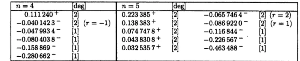
Wewrite anexamplefor $N=10$ and $\Delta=-1/2$, with the choice of $z,$$y,$$\rho$ as inthe left column

ofTable 1. After diagonalizing numerically the blocks $n=4,5$ of the transfer matrix, theeigenvalues

corresponding to bound pairs (we have recognized them because they match exactly

our

predicted

values)$\mathrm{a}\mathrm{p}\mathrm{n}\mathrm{r}\mathrm{o}\mathrm{x}\mathrm{i}\mathrm{m}\mathrm{a}\mathrm{t}_{}\theta \mathrm{d}$ tothe $\mathrm{n}\Leftrightarrow \mathrm{a}\mathrm{r}\mathrm{p}..\mathrm{q}\mathrm{t}.$six $\mathrm{d}\mathrm{i}\sigma \mathrm{i}\mathrm{f},$ $\mathrm{n}\iota\iota \mathrm{r}\mathrm{n}\mathrm{b}_{6\mathrm{r}\mathrm{a}YP}..24$

:

Table2. Eacheigenvaluelisted isfollowedbyasign $+\mathrm{o}\mathrm{r}$ –: the sign $+\mathrm{i}\mathrm{n}\mathrm{d}\mathrm{i}\mathrm{c}\mathrm{a}\mathrm{t}\mathrm{e}\mathrm{s}$that _{$e_{1}e_{2}e_{3}e_{4}=1$} (orthat $e_{1}e_{2}\epsilon_{3}\epsilon_{4}\mathrm{e}_{6}=1$

if $n=5$),the sign –that theproductof the Betherootsis $-1$

.

The degeneration of the eigenvalue is$[\deg]$. In the column

corresponding to $n=4$,the number 0.111240 coincides with (8.13), andthe remainingfive values agreewiththe theoretical

A obtainedinserting(8.14)and(8.15)into(5.3). Theeigenvalue that corresponds to $r=-1$,remember thatin this column $r$

isasolutionof(8.8), is degenerated. $\mathrm{T}\mathrm{h}\dagger \mathrm{s}$degenerationis

notasurprise, because it$is$acasein which two Bethe roots coincide

$(e_{3}=e_{4}=-1)$ , and whenit is true that the eigenvector associatedtosuchcasesisusually thezerovector, when $\Delta=-1/2$

it is not. Regardingthe list when $n=5$ ,the values with a $+$ correspond to solutions $r$ of(8.10), and thevalueswitha

-tosolutions $r$ of thepolynomial thatisobtained changing in (8.10)the variables $r,$$\Delta$ by

$-r,$$-\Delta$

.

Totally expected is

thedegenerationof the eigenvalue -0.0869220 since $e_{3}=e_{4}=-1,$$e\mathrm{s}=1$. But the degeneration of -0.0657464 which

happensfor $e_{3}=-2,$$\epsilon_{4}=-1/2,$_{$e_{6}=-1$} islessexpected.

The last comment ofthe paper: the numerators of (6.1), (7.5), (8.12), (8.14) and (8.18)

are

polyno-mials in $z$ with

a

reciprocal property: if $R$ is

a

solution,

so

it is $1/R$

.

When lookingfor other $Q’s$ in

$n=7$ (say)

one

has to restricttonumerators withthis property. Acknowledgments

I am pleased to thank Prof. J. Shiraishi and the organizers of the RIMS 2004 Symposium, Recent

progressin Solvable LatticeModels, held in Kyoto forallowing meto exposethese ideas. Inmywork

I amgrateful to G.

Alvarez

Galindo for resolving some of mydoubts. But to whom I feel inevitably

grateful every day is to Pepe Aranda: seventy times

seven

I have knocked

on

his door asking about

polynomials, roots andother mattersof Calculus, andseventy times

seven

he has received

me

without

ever

showing the slightest unwelcomegesture in his face

or manners

that prevented

me

from knocking

on

hisdoor again.

Thisworkis financially supported bythe Ministerio de Educacio’n $\mathrm{y}$Cienciaof Spainthrough grant

No. BFM2002-00950.

References

[1] R.J. Baxter, Completeness

_of

he Bethe ansatz

_for

the six and eight-vertex models, J. Statist. Phys. 108

(2002) 1.cond-mat/0111188.

[2] H. Bethe, Zur Theorie derMetalle,Z. Physik 71 (1931)205. English translation: On thetheory

_of

metals, I: Eigenvalues and eigenfunctions

_of

alinearchain

_of

atoms in “The many-body problem”,ed.D.C. Mattis, WorldScientific,Singapore, 1993. pages 689-716.

[3] R. Siddharthan, $Singu\iota_{af};ties$ in the Bethe solution

of

the XXX and XXZ Heisenberg spin chains, cond-mat/9804210.

[4] J.D. Noh, D-S. Lee and D. Kim, Origin

_of

the $sin\phi ar$Bethe ansatzsolutions

for

the Heisenberg XXZ

spin chain, PhysicaA287 (2000) 167.$\mathrm{c}\mathrm{o}\mathrm{n}\mathrm{d}-\mathrm{m}\mathrm{a}\mathrm{t}/\mathfrak{M}1175$.

[5] M.T. Batchelor,Finite latticemethods in statistical mechanics,Ph.D.thesis,Australian NationalUniversity,

Canberra, 1987.

[6] N. Beisert, J.A.Minahan,M. Staudacher and K. Zarembo, StringingSpins andSpinning Strings,JHEP09 (2003) 010. hep-th/0306139.

[7] T. Fujita, T. Kobayashi and H. Takahashi, Large $N$ behavtor

of

string solutions in the Hersenberg model,

J. Phys. $\mathrm{A}$: Math. Gen. 36 (2003) 1553. cond-mat/0207117.

[8] E.H. Lieb, Exact solution

_of

the problem

of

the entropy

_of

two-dimensionalice, Phys.Rev. Lett. 18 (1967) 692; Residual entropy

_of

square ice, Phys. Rev. 162 (1967) 162. B. Sutherland, Exact solution

_of

a two-dimensional model

_for

hydrogen-bonded crystals, Phys. Rev. Lett. 19(1967) 103. C.P. Yang, Exactsolution

of

amodel

_of

two-dimensional

_{ferroelectrecs}

inanarbrtraryexternalelectrec field, Phys. Rev. Lett. 19(1967)

586.B. Sutherland,C.N. Yang andC.P.Yang, Exact solution

_of

a model

_of

two-dimensional$feffoelect;\dot{\backslash }cs$

in anarbitrary external fidd, Phys. Rev.Lett. 19(1967) 588.

[9] R.J. Baxter,Exactlysolvedmodels in statisticalmechanics,AcademicPress, London,1982. [10] J.V. Uspensky, Theory

of

equations, McGraw-HiU, NewYork, 1948.