A portfolio model for the risk management in public pension (Financial Modeling and Analysis)

A

portfolio

model for

the

risk

management

in

public

pension*

Tadashi Uratani

Department of System Engineering Hosei University

Abstract

The financial sustainability of public pension requires the reserve should be positive

to pay the benefit in the demographic and economical environment change subject to the

certain level of the income replacement ratio. Assuming the market asset and the income

for pension follows Ito processes and we maximize the net present value of pension for the

cohort, To guarantee the pension fund sustainability, we apply the martingale method of

the optimal consumption and investment theory. We use the age-structured model to the

pension population change.

Keywords: public pension, portfolio risk management, population cohort

1

Introduction

1.1

Risk management for

a

public pension

Welfare nationshave beensuffering therobust managementofpublic pension

as seen

thereform

in [4] and [5]. Japanese government has announced every five years the actuarial valuation of

pension plan for 100years,

as seen

[6]. It reviewed the longterm financial viability under

signif-icant changes in the demographic and economical environment. The financial viability implies

that the

reserve

of pension fund should be positive, under the $co$ndition that the replacement

ratiois

more

the50

%,

which

means

thatthe

average

amountofpensionis

more

than the average

income of contributors.

The aging society with the low birth ratemakesworsethe balance ofpensionaccount inthe

near future withthe prolonged deflationary economy in Japan.

Economic scenarios for the simulation are the rate of return of investment, the wage as the

key factorof contribution and benefit, andinflation rate and interest rate.

The total pension fund

was

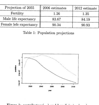
144.4 trillion yen at 2009 and has decreased to 120 trillion at

2012. There exists the ambiguity in population projection by Government survey [6] as Table

1.1. Figurel.1 is the governmental projections ofpopulations ofpension.

The long term economic scenarios

were

assumed

as

Tablel.1. In2004thegovernment reform

plan hadset the maximum premiumrate

as

18.3% and benefit cutoffby the rate ofdecreasing

contributors and aging rate. Their plan starts from 2012 and will end

2038.

1.2

$A$ portfolio

formulation for pension

risk

management

The objective satisfies the following considerations; 1) to minimize the government subsidy

to pension fund, 2) to maximize the net present value of pension premium and benefit, 3) to

’This researchwassupportedinpart bytheGrant-in-Aid for Scientific Research(No. 25350461) of theJapan

Table 1: Population projections

yeer

Figure 1: contributors$(-)$ _and beneficiaries $($ — $)$

minimize thedifferenceamonggenerations in the net values, 4) to perform income redistribution to the poor elderly.

The constraints are followings; 1) no default of pension system for 100years, 2) The

reserve

fund at the end ofplan should be enough to continue the system. 3) The income replacement

ratio should be

more

than 50%.

2

The model

2.1

Policyholders

Let $p(t, y)$ denote _{the numbers of policyholders of the age}

$y$ at $t$ and

$\omega_{1}$ the starting age of

paying premium, $\omega_{2}$ the end ageand starting of receiving benefit

$\omega_{3}$ the end age of beneficiary.

The total number of contributors satisfies:

$\xi_{t}^{1}=\int_{\omega_{1}}^{\omega}2p(t, y)dy$ (2.1)

Thetotal number ofbeneficiaries:

$\xi_{t}^{2}=\int_{\omega 2}^{\omega 3}p(t, y)dy$ (2.2)

The balanceof total premium and benefit is assumed to bebased

on

the average wage. Let

$H_{t}$ denote the average wage at $t$ and $a_{t}$ be the rate ofpremium. Let $u_{t}$ be the total premium

amount at $t$;

$u_{t}:=a_{t}H_{t}\xi_{t}^{1}$

Let $b_{t}$ be the benefit ratio to the average wage and $s_{t}$ be thetotal benefit amount;

$s_{t}:=b_{t}H_{t}\xi_{t}^{2}.$

We

assume

that $a_{t},$$b_{t}$ is predictable process and it satisfies self-finance strategies, which

are

in

the condition of$0<a_{t},$ $b_{t}<1$

.

The balance of premium and benefit $q_{t}(a, b)H_{t}$ is defined as: $u_{t}-s_{t}=(a_{t}\xi_{t}^{1}-b_{t}\xi_{t}^{2})H_{t}=:q_{t}(a, b)H_{t}.$

2.2

The portfolio

The pension portfolio consists of three assets; Market asset price satisfies the following It\^o

process:

$dA_{t}/A_{t}=\mu_{r}(t)dt+\sigma_{r}(t)dW_{t}^{r}=:dr_{t},$

Humancapital price(wage) process satisfies:

$dH_{t}/H_{t}=\mu_{x}(t)dt+\sigma_{x}(t)dW_{t}^{x}=:dx_{t},$

The riskfree rate $r$ and the money market account $e^{rt}.$

Portfoliostrategies ofthe pension fund

are

denoted

as

$\pi_{t}:=(\phi_{t}, a_{t}, b_{t},\beta_{t})$; Let $\phi_{t}$ denote the

investment amount ofmarket asset, $(a_{t}, b_{t})$ denote the strategies for the human capital which

means the policy of pension. Let $\beta_{t}>0$ denote the government subsidy to pension fund at $t$

and $R_{t}$ denote the value ofpension fund at $t.$

The portfolio valuesatisfies at $t$:

$R_{t}=\phi_{t}A_{t}+q(a, b)H_{t}$ (2.3)

The dynamics offund is due to the predictability ofstrategies $(\phi_{t}, \beta_{t})$:

$dR_{t}=\phi_{t}dA_{t}+d(q(a, b)H_{t})+\beta_{t}dt, R_{0}=\overline{R}$ (2.4)

The population dynamics is assumed to be non stochastic but not satisfies self financing

condition then the dynamics of the balance of premium and benefit of pension is as follows,

$d(q(a, b)H_{t}) = a_{t}(d\xi_{t}^{1}H_{t}+\xi_{t}^{1}dH_{t})-b_{t}(d\xi_{t}^{2}H_{t}+\xi_{t}^{2}dH_{t})$

Letdefine the change of balancedue to changeof numbers ofcontributors and beneficiaries;

$dq(a, b)$ $:=a_{t}d\xi_{t}^{1}-b_{t}d\xi_{t}^{2}$, then

$d(q(a, b)H_{t})=q(a, b)dH_{t}+dq(a, b)H_{t}.$

Subsitute it to (2.4) then

$dR_{t}=\phi_{t}A_{t}dr_{t}+q(a, b)H_{t}dx_{t}+dq(a, b)H_{t}+\beta_{t}dt.$

By using (2.3) we obtain:

$dR_{t}=R_{t}dr_{t}+q(a, b)H_{t}(dx_{t}-dr_{t})+dq(a, b)H_{t}+\beta_{t}dt.$

From (2.1) and(2.2),

$dq(a, b) = a_{t}d\xi_{t}^{1}-b_{t}d\xi_{t}^{2}$

$= \{a_{t}\int_{\omega_{1}}^{\omega_{2}^{-}}\frac{\partial p(t,y)}{\partial t}dy-b_{t}\int_{\omega_{2}}^{\omega_{3}}\frac{\partial p(t,y)}{\partial t}dy\}dt$

From the PDE ofMcKendrick-von Foerster

$\frac{\partial p(t,y)}{\partial t}=-\frac{\partial p(t,y)}{\partial y}-\mu(t, y)p(t, y)$, (2.5)

where $\mu(t, y)$ is decreasing speed ofpension participant at $t$of the age

$y.$

2.3

The cohort

modeling

Weusethemethod ofcharacteristicsin PDE whichequalstouse the cohort model ofpopulation.

Let $t=k+y$ and

assume

$\mu(y)=\mu(t, y)$ which

means

_{the decreasing number depends only}

the age. Let $v(k, y)$ $:=p(t, k)$ then From (2.5) we get:

$dv(k, y)=-\mu(y)v(k, y)dy.$

and thesolution is

$v(k, y)=v(k, 0) \exp(\int_{0}^{y}\mu(s)ds)$

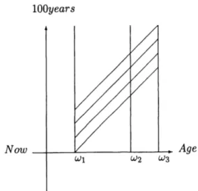
In Figure 2.3 is seen the cohort model in a public pension plan for 100 years horizon and the

ages ofcontribution $(\omega_{1}, \omega_{2})$ and benefit $(\omega_{2}, \omega_{3})$

.

The change of contributor is from (2.1):

$d \xi_{t}^{1} = -\int_{\omega_{1}}^{\omega_{2}^{-}}\mu(y)v(k, y)dy,$

andthe change ofbeneficiaries is similarily:

$d \xi_{t}^{2} = -\int_{\omega_{2}}^{\omega_{3}}\mu(y)v(k, y)dy.$

Thus the change of pension balance satisfies ;

$dq_{t}(a, b)H_{t} = (a_{t}d\xi_{t}^{1}-b_{t}d\xi_{t}^{2})H_{t}$

$= -(a_{k+y} \int_{\omega_{1}}^{\omega_{2}^{-}}\mu(y)v(k, y)dy-b_{k+y}\int_{\omega}^{\omega_{3}}2\mu(y)v(k, y))H_{t}$, (2.6)

where$p(k+\omega_{1}, \omega_{1})$ is the

new

entry numbers of contributors and

$p(k+\omega_{2}, \omega_{2})$ isthe

new

entry

$100years$

Figure 2: Cohorts and 100 year pension plan

3

The

pension strategies

3.1

The present

value of pension

for

a

cohort

For thetimehorizon from$0$ to$T$there

are

$k$cohort of$0\leq k\leq T_{l}$ $:=T-(\omega_{3}-\omega_{1})$who

are

their

all contributions and benefits

are

within the planning period. These cohorts

are new

comers

to

the pension.

$c(k) :=- \int_{\omega_{1}}^{\omega_{2}^{-}}a_{y+k}H_{y+k}^{*}v(k, y)dy+\int_{\omega}^{\omega_{3}}2b_{y+k}H_{y+k}^{*}v(k, y)dy$ (3.1)

For existing pensionaries $(-\omega_{3}<k<0)$

,

their premium and benefit

was

decided as $a_{c}$ and $b_{c}$ for the past $:y+k<0$; They will follow the

new

premium and benefit from

now

$y+k\geq 0.$

The net present value $c_{e}(k)$ should be positive;

$c_{e}(k)=- \int_{\omega}^{\omega_{2}^{-}}1(a_{c}1_{\{y+k<0\}}+a_{y+k}1_{\{y+k\geq 0\}})H_{y+k}^{*}v(k, y)dy$

$+ \int_{\omega}^{\omega 3}2(b_{c}1_{\{y+k<0\}}+b_{y+k}1_{\{y+k\geq 0\}})H_{y+k}^{*}v(k, y)dy$

.

(3.2)

For the future cohort $(T_{l}<k<T)$ whosebenefit willnot finished before$T$, their net present

value $c_{p}(k)$ should be positive;

$c_{p}(k)=- \int_{\omega_{1}}^{\omega_{2}^{-}}(a_{k+y}1_{\{y+k<T\}}+\tilde{a}_{y+k}1_{\{y+k\geq T\}})H_{y+k}^{*}v(k, y)dy$

$+ \int_{\omega}^{\omega_{3}}2(b_{y+k}1_{\{y+k<T\}}+\tilde{b}_{y+k}1_{\{y+k\geq T\}})H_{y+k}^{*}v(k, y)dy$

.

(3.3)

The past balance ofpremium and benefit are accumulated

as

a part of the present reserve

fund $R_{0}$;

problem of public pension

The objective function is to maximize the utility function of the new pension participant who

are the cohort of $0\leq k\leq T_{l}$, where $U_{1}$$(.$$)$ is a utility function for present value ofpension and $U_{2}(\cdot)$ is the utility of fund value at $T$:

$\max_{\pi_{t}}E[\int_{0}^{T_{l}}U_{1}(c(k)dk+U_{2}(R_{T})]$

Beside constraints (3.2) and (3.3), we impose the following constraints seen in [5];

(1) No default of pension fund, whichshould satisfiesthe following;

$R_{t}>0 \forall t\in[0, T],$

(2) Government subsidy $\gamma_{t}$ should be within the limitation;

$E^{Q}[ \int_{t}^{T}e^{-rs}\beta_{s}ds|\mathcal{F}_{t}]\leq\gamma_{t}.$

At the planning time it is as follows;

$E^{Q}[ \int_{0}^{T}e^{-rs}\beta_{s}ds]\leq\gamma_{0}$

(3) The economic rationality to hold the pension; For the existing policyholders;

$E^{Q}[c_{e}(k)]>0, k\in(-\omega_{3},0)$

For the future policyholders;

$E^{Q}[c_{p}(k)]>0, k>T-(\omega_{3}-\omega_{1})$

4

Pension

portfolio

process under the risk

neutral

probability

4.1

Martingale method

for

the

risk

management

Theriskmanagement ofpensionshould be no defaultwhichimpliesthat $R_{t}>0$for all$t\in(0, T)$

.

It can be treated by the martingale method ofoptimal investment and consumption problem of

Dana-Jeanblanc $[2],ppl37-144.$

Let $e^{rt}$ a numeraire, from (2.3) and (2.4)

$dR_{t}e^{-rt}-R_{t}re^{-rt}dt=(\phi_{t}dA_{t}+q(a, b)dH_{t}+dq(a, b)H_{t}+\beta_{t}dt)e^{-rt}-(\phi_{t}A_{t}+q(a, b)H_{t})re^{-rt}(4.1)$

Then

$d(R_{t}/e^{rt})=\phi_{t}d(A_{t}/e^{rt})+q(a, b)d(H_{t}/e^{rt})+dq(a, b)H_{t}e^{-rt}+\beta_{t}e^{-rt}dt$

Let denote $R_{t}^{*}:=R_{t}/e^{rt},$ $A_{t}^{*}=A_{t}/e^{rt},$ $H_{t}^{*}=H_{t}/e^{rt}$, then

$dR_{t}^{*}=\phi_{t}dA_{t}^{*}+q(a, b)dH_{t}^{*}+dq(a, b)H_{t}^{*}+\beta_{t}e^{-rt}dt$ The

reserve

fund at $T$ becomes as follows:

$R_{T}^{*}=R_{0}+ \int_{0}^{T}\phi_{t}dA_{t}^{*}+\int_{0}^{T}q(a, b)dH_{t}^{*}+\int_{0}^{T}H_{t}^{*}dq(a, b)+\int_{0}^{T}\beta_{t}e^{-rt}dt$, (4.2)

4.2

The admissible

strategies

The admissible strategies satisfying the constraint $R_{t}>0$

as

Dana et al [2]. We

assume

that

the government subsidy to the pension fund shouldsatisfies $E^{Q[} \int_{t}^{T}\beta_{s}ds+\int_{t}^{T}H_{s}dq(a, b)]\leq 0.$

It is theassumption that the government subsidy is less than the deficit due to the population change oftheaging with low fertility. Anotherassumptionwhichis taken fromJapanese pension report isthat the final

reserve

fund

covers

the pension benefit;

$R_{T}=H_{T}b_{t}\xi_{t}^{2}$ (4.3)

From (4.2)

$R_{t}^{*}- \int_{0}^{t}H_{s}^{*}dq(a, b)-\int_{0}^{t}\beta_{t}e^{-rs}ds=R_{0}+\int_{0}^{t}\phi_{s}dA_{s}^{*}+\int_{0}^{t}q(a, b)dH_{s}^{*}=:M_{t}$ (4.4)

$M_{t}$ isa positive $Q$-martingale which is under the risk neutral probability. Then

$R_{t}^{*}=M_{t}+ \int_{0}^{t}H_{s}^{*}dq(a, b)+\int_{0}^{t}\beta_{t}e^{-rs}ds$ (4.5)

Using the conditional expectation ofthe martingale

$R_{t}^{*}$ $=$

$\frac{E^{Q}[R_{T}^{*}-\int_{0}^{T}H_{s}^{*}dq(a,b)-\int_{0}^{T}\beta_{s}e^{-rs}ds|\mathcal{F}_{t}]}{M_{t}}+\int_{0}^{t}H_{s}^{*}dq(a, b)+\int_{0}^{t}\beta_{S}e^{-rs}ds$

$= E^{Q}[R_{T}^{*}-l^{\tau_{H_{t}^{*}dq(a,b)}}-l^{T}\beta_{t}e^{-rs}ds|\mathcal{F}_{t}]$

From the assumption $E^{Q[} \int_{t}^{T}\beta_{s}ds+\int_{t}^{T}H_{s}dq(a, b)]\leq 0.$ $H_{t}^{*}$ is $Q$-martingale then $E^{Q}[H_{T}^{*}]=$

$H_{0}>0$

.

Therefore the theterminal

reserve

$E^{Q}[R_{T}^{*}]>0$ by (4.3). From these two conditions $R_{t}>0, \forall t\in(0, T)$

and

$E^{Q}[R_{?}^{*}- \int_{0}^{T}H_{s}^{*}dq(a, b)]\leq B_{4}+\gamma 0$

We restate the above

as

the following theorem;

Theorem 1

_if

$E^{Q[} \int_{t}^{T}\beta_{s}ds+\int_{t}^{T}H_{s}dq(a, b)]\leq 0$ and

if

the

final

reserve

satisfies

$(4\cdot 3)$

,

then

$R_{t}>0, \forall t\in(0, T)$

4.3

The optimal problem

From theconsequenceof (4.3), set the objectivefunction as

$\max_{\pi_{t}}E[\int_{0}^{T_{l}}U_{1}(c(k))dk].$

Thefirst constant is

$E^{Q}[R_{T}^{*}- \int_{0}^{T}H_{s}^{*}dq(a, b)]\leq R_{0}+\gamma_{0}.$

Define the Radon-Nikodim derivative for the risk neutral measure: $L_{t}=dQ/dP|_{\mathcal{F}_{t}}$ then the

constraint becomes under the original probability measure;

$E[L_{T}R_{T}^{*}- \int_{0}^{T}L_{t}H_{s}^{*}dq(a, b)]\leq R_{0}+\gamma_{0}$

The third constraints are For the existing policyholders;

$E^{Q}[c_{e}(k)]>0, k\in(-\omega_{3},0)$

For thefuture policyholders;

$E^{Q}[c_{p}(k)]>0, k>T-(\omega_{3}-\omega_{1})$

This optimal problem willbe solved in discretized version.

References

[1] Clark, C. W.,(2010): Mathimatical Bioeconomics, John Wiley

[2] Dana,R-A., Jeanblanc, M.,(2007): Financial Markets in Continuous Time,Springer Finance

[3] Kot, M.,(2001): Elementsof Mathematical ecology, Cambridge University press

[4] Bundesministerium f\"ur Albert und Soziales,(2005):

\"Uberblick

\"uber das Sozialrecht

[5]

WAifltf

$\{\Phi’k^{\backslash }ffi\ovalbox{\tt\small REJECT} \mathscr{X}\Phi^{\overline{\overline{-}}}\ovalbox{\tt\small REJECT},$ $*\pi$2 $1\not\in \mathbb{R}ffli\mathfrak{N}\Re_{I}^{\overline{E}}g\varphi_{\mathfrak{o}^{b}}\ovalbox{\tt\small REJECT}\triangleright,\dagger^{o}\backslash -k$

[6] $\ovalbox{\tt\small REJECT}\xi E9?\ovalbox{\tt\small REJECT}’g^{\backslash }\not\in\Leftrightarrow\ovalbox{\tt\small REJECT} \mathscr{X}\Phi^{-}\ovalbox{\tt\small REJECT},$ $\ovalbox{\tt\small REJECT}\#\not\in\not\in\cdot$

Department of System Engineering

Faculty ofScience

&

Engineering

Hosei University, Koganei 184-8485, Japan

$E$-mail address: uratani@hosei.ac.jp

$\mathfrak{F}\infty X\ovalbox{\tt\small REJECT}$

.

$\Phi$エ$\neq$P $*$

\S