On the Convergence of the Jacobi-Davidson Method - Based on a Shift Invariance Property (Mathematical foundation and development of algorithms for scientific computing)

On the

Convergence

of

the

Jacobi-Davidson Method

-

Based

on a

Shift

Invariance

Property

名古屋大学大学院工学研究科 宮田 考史 (Takafumi Miyata)

Graduate SchoolofEngineering, Nagoya University

愛知県立大学大学院情報科学研究科 曽我部 知広 (Tomohiro Sogabe)

Graduate School ofInformationScience& Technology, Aichi Prefectural University

名古屋大学大学院工学研究科 張 紹良 (Shao-Liang Zhang)

Graduate School ofEngineering, NagoyaUniversity

Abstract

Jacobi-Davidson type methods have been recently proposed for the

iter-ative compution ofafeweigenpairs ofalarge-scale andsparse matrix. This

type methods are characterized by the correction equation for generating

a subspace where eigenpairs are approximated. In this report, we present a

shiftinvariancepropertyof the Krylov subspaceon aprojectedspace. Based

ontheproperty, aprocedureforsolving thecorrection equation is proposed.

Through theprocedure, we canconstructnot onlyexistingmethods but also

new methods ofJacobi-Davidsontype.

1

Introduction

Given

an

$N\cross N$ large and sparse matrix $A$, we considercomputing a few

eigen-pairs $(\lambda\in \mathbb{C},x\in \mathbb{C}^{N})$ satisfying

$A$$x=\lambda x$ $(x\neq 0)$. (1) For the iterative computation ofeigenpairs, Krylov subspace methods are widely

used, e.g., the Lanczos method [7, 2] (when $A$ is Hermitian) and the Amoldi

method [1, 2] (when $A$ is non-Hermitian). On the other hand,

a

different type

ofiterative methods have been recently proposed, e.g., the Jacobi-Davidson (JD)

method[10, 5, 2] and theRiccati method [3]. This typemethods

are

characterized by the correction equation [10] forgenerating a subspace. Here, we focus on this

type methods and call them JD-type methods.

InJD-typemethods,the correction equationis(approximately)solved for

gen-erating

a

basis vector ofa subspace. According to solvers for the equation, dif-ferent subspaces

are

generated, i.e., different JD-type methods

are

produced. In this report,

we

present a shift invariance property of the Krylov subspace

on a

equation is proposed. Through the procedure, not only existing JD-type

meth-ods but also

new

JD-type methods

can

be constructed. Relationship

among

the

constmcted methods

are

established.

This report is organized

as

follows. In section 2,

we

describe the correction equation in JD-type methods. In section 3, we present

our

procedure for solving the correction equation. Through the procedure, JD-type methods

can

be

con-stmcted. In section 4, numerical experiments

are

reported to

compare

JD-type methods. Finally,

we

summarize this report in section 5. Throughout this report,

$I$ denotes the $N\cross N$ identity matrix, and$(\cdot)^{*}$ denotestheconjugatetranspose. Let

$(K_{m}(A, b)$ denote the m-dimensional Krylov subspace span_{$\{b, Ab, ..., An-1b\}$}.

2

JD-type

methods

To start with,

we

describe the colTection equation in JD-type methods. The equa-tion is a reformulation ofJacobi’s idea [6] for generating

a

subspace. Then, the JD method and the Riccati method are outlined.

2.1

The

correction

equation

Let $Q$ be an $N\cross k$ matrix whose column vectors form an orthonormal basis of

a subspace $O$. Let $(\theta, u)$ be an approximate eigenpair. We consider $u\in O$, i.e.,

$u=Qy(y\in \mathbb{C}^{k})$. The Rayleigh quotient of $u$ is taken as the approximate

eigenvalue $\theta=u^{*}Au$ with _{$||u||_{2}=1$.} We define the residual vector _{$r=Au-\theta u$}

and compute $\Vert r||_{2}$ to checkthe

accuracy

of$(\theta, u)$.

Here, we are given the approximate eigenpair$(\theta, u)$ to $(\lambda, x)$. To get the exact

eigenvector $x$, Jacobi’s idea is to find the correction vector $t=x-u$ satisfying $t\perp u$. From Eq. (1), $t$ satisfies

$A(u+t)=\lambda(u+t)$. (2)

Let$P=I-uu^{*}$_{, then applying the projector}$P$ to Eq. (2) leads to the correction

equation [10] as follows

$P(A-\lambda I)Pt=-r$. (3)

The unknown eigenvalue $\lambda$ exists in Eq. (3). To vanish 1, the projector $I-P$ is applied to Eq. (2). This leads to

$\lambda=u^{*}Au+u^{*}A$ $t$. (4)

From Eqs. (3) and (4), a Riccati form [3] of the correction equation is derived as follows

In JD-type methods, the correctionvector $t$ is approximated and the

approxi-mationisusedto expand the subspace$O$. In the expanded subspace, the eigenpair

will be approximated again.

2.2

Solving the

correction equation

Two JD-type methods

are

briefly described here. One is the Riccati method, the

other is the JD method.

The Riccati methodapproximates the solutionvectorofnonlinearequation (5)

in

a

Krylov subspace [3]. On the other hand, typically in the JD method, Eq. (5)

is linearized and the following linear system

$P(A-\theta I)Pt=-r$ (6)

is approximately solved by the GMRES algorithm [9]. The JD method discards the term $u^{*}At$. From this difference, the Riccati method may show faster

conver-gence than the JD method.

3

Constructing JD-type

methods

Ourapproach for computingthe correctionvector is outlined as follows.

$\bullet$ Replace the unknown eigenvalue $\lambda$in Eq. (3) by its approximation $\sigma$.

$\bullet$ Solve the following linear system

$P(A-\sigma I)Pt=-r$. (7)

To this end, double Krylov subspaces

are

used

as

follows.

$\bullet$ The first subspace $’\kappa_{m}(A, u)$ for$\sigma$.

$\bullet$ The secondsubspace$’\kappa_{l}(P(A-\sigma I)P, r)$ forsolving Eq. (7)approximately.

3.1

Shift

invariance property

The computational cost of the approach is considerable, especially in

matrix-vector multiplications for generating the basis vectors of the double Krylov

sub-spaces.

To

save

thesecosts,

we

make clear

a

relationship of the subspaces.

Itis known that the Krylov subspace is shift invariant, i.e.,

$’\kappa_{n}(A-\sigma I, b)=’\kappa_{n}(A, b)$. We show that the property holds ona projected space [8].

Theorem 1 Let $G$ be an $N\cross N$ matrix satisfying _{$G^{2}=G,$ $G^{*}=G.$} Then, the

Krylov subspace on aprojectedspace is

_shift

invariant, _{that is}

$j\zeta_{n}(G^{*}(A-\sigma I)G, Gb)=’\kappa_{n}(G^{*}AG, Gb)$. ₍₈₎

Corollary 1 From Eq. (8), _{the double Krylov subspaces satisfy}

$’\kappa_{n}(P(A-\sigma I)P, r)=PK_{n+1}(A, u)$. ₍₉₎

From Eq. (9), the basis ofthe first subspace

can

be reused as that ofthe second

subspace. The computational cost for generating the basis are therefore saved.

3.2

Procedure

for the

correction equation

By utilizing the _{relationship ofthe double Krylov subspaces,}

_our

_{approach is}

out-lined as follows.

Krylov procedure for the correction equation (7)

Step 1. Setparameters $m,$ $n$, and $f= \max(m, n+1)$.

Step 2. Generate $\ell$-orthonormal basis

vectors $v_{1},$ $\ldots$ ,$v_{C}$ of $’\kappa_{p}(A, u)$.

Step 3. Setthe algorithmto generate the approximate eigenvalue $\sigma$ in

$7C_{m}(A, u)=$ span$\{v_{1}, \ldots, v_{m}\}$.

Step 4. Setthe algorithmto solve Eq. (7) approximately in

$(K_{n}(P(A-\sigma I)P, r)=$ span$\{v_{2}, \ldots, v_{n+1}\}$.

Through the procedure, JD-type methods

can

be constmcted by the decision of

the parameters, i.e., $m,$ $n$ and the two algorithms at Steps 3 and 4. Examples of

the constructed methods

are

shown in Table 1.

Table 1: The parameter decision forJD-type methods.

$\frac{Type|m|A1gorithmatStep3|A1gorithmatStep4}{|\begin{array}{l}\overline{1}+n1+n1+n1\end{array}|}(((II)Amo1di(Ritz)$

Remark 1 Suppose the$JD$ methodisset upwith then-steps

of

the GMRES algo-rithm

_for

solving Eq. (6)

approximately.

Then, _the$JD$ methodis equivalent to the JD-type (I) methodin Table 1.

Remark 2 Suppose theRiccati method is set up with the n-dimensional Krylov subspace

_for

solving Eq. (5)approximately. Then, the Riccati methodisequivalent

to theJD-type (II) methodin Table 1.

Fromthe above remarks, we compare the JD method with theRiccati method. At Step 2 in the Krylov procedure, $f=n+1$ dimensional subspace is generated

in the both methods. At Step 3, the JD method utilizes only $m=1$ dimensional

subspace whereas the Riccati methodutilizesthe

maximum

$m=n+1$ dimensional

subspace. Hence, in the Riccati method, a better approximate eigenvalue $\sigma$

can

be set in Eq. (7). As

a

result, a better approximation of the correction vector

maybe produced inthe Riccati method. Forthis reason, the Riccati method may

show faster

convergence

than the JD method. However, inthe Riccatimethod, the Amoldi algorithm producing Ritz values is implicitly used at Step 3. This

may

not be appropriatewhendesired eigenvalues

are

interior.

We consider constmcting other JD-type methods, e.g., Type (III) and (IV) in

Table 1. The parameter $m$ is the

same as

that in the Riccati method to utilize

the maximum dimensional subspace at Step 3 for approximate eigenvalues. In

the Amoldi algorithm at Step 3, Ritz values

are

produced forexterioreigenvalues

(Type (III)) whereas harmonic Ritz values

are

produced for interior eigenvalues

(Type (IV)). To produce the minimum residual solution of Eq. (7), the shifted

GMRES algorithm is adopted at Step 4 (Type (III) and (IV)).

4

Numerical

experiments

We show numerical experiments to compare the three kinds of JD-type methods.

The JD method approximately solved Eq. (6)by the $n=10$ _{steps of the GMRES}

algorithm. The Riccati method approximatelysolved Eq. (5) in the$n=10$

dimen-sional Krylov subspace. The JD-type (III) method approximately solved Eq. (7)

with the parameter$n=10$. Number ofmatrix-vectormultiplications

per

iteration

were the

same

in all the methods.

By using these methods,

_we

computed the largest eigenvalue and its

corre-sponding eigenvector of the real nonsymmetric matrix DW8192 obtained from

[4]. These experiments

were

implemented with Fortran 77 in double precision arithmetic on AMD Phenom 9500 (2.2 GHz). In the three methods,

an

ini-tial approximate eigenvector was given by a common vector whose elements

were random numbers. Iteration

was

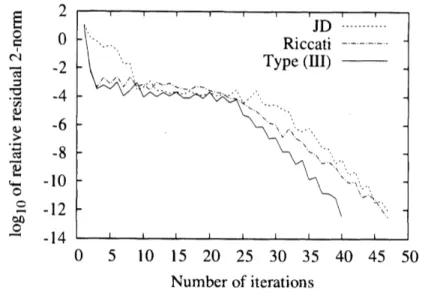
stopped when the relative residua12-norm

$\frac{\circ tfg\not\in 1}{l,3}Q\frac{\varpi}{\omega}$ $\frac{.\dot{63}\underline{\circ>}}{\omega}$ $u_{O}$ $\frac{c}{\alpha),\underline{\circ}}$ $0$ 51015 20 25 30 35 40 45 50 Numberofiterations

Figure 1: Convergence histories ofrelative residua12-norms.

As shown in Figure 1, the Type (III) method showed faster

convergence

than

both the JD method and the Riccati method. With respect to computational time, the JD method required 2.17 seconds, the Riccati method required 2.25 seconds,

and the Type (III) method required 1.60 seconds.

5

Conclusion

In this report, we

presem

a shift invariance property ofthe Krylov subspace

on

a projected space. By utilizing the property, we provide a procedure for solving

the correction equation. Through the procedure, not only existing JD-type meth-ods but also new JD-type methods can be constmcted. Numerical experiments

indicates that the new JD-type method is a good competitor to existing JD-type methods.

References

[1] W. E. Amoldi, The principle of minimized iteration in the solution of the

matrix eigenvalue problem, Quart. Appl. Math., 9 (1951), 17-29.

[2] Z. Bai, J. Demmel, J. Dongarra, A. Ruhe, and H.

van

der Vorst, eds.,

Tem-plates

_for

thesolution

_ofA

lgebraic EigenvalueProblems.$\cdot$

A Practical Guide,

SIAM, Philadelphia,2000.

[3] J. H. Brandts, The Riccati algorithm for eigenvalues and invariant subspaces

ofmatrices with inexpensiveaction, LinearAlgebraAppl., 358 (2003), 335-365.

[4] T. Davis, The University of Florida SparseMatrix Collection,

http:$//www$

.

cise. ufl. edu/research/sparse/matrices.

[5] D. R. Fokkema, G.L.G. Sleijpen, and H. A.

van

der Vorst, Jacobi-Davidson styleQRandQZ algorithmsforthe reduction ofmatrix pencils, SIAMJ Sci.

Comput., 20 (1998), 94-125.

[6] C. G. J. Jacobi, Ueber ein leichtes Verfahren, die in der Theorie der S\"acularst\"omngen vorkommenden Gleichungen numerisch $aufzulsen,$ $J$

ReineAngew. Math., (1846), 51-94.

[7] C. Lanczos, An iteration method for the solution of the eigenvalue problem

of linear differential and integral operators, $J$ Res. Nat. $Bur$. Standards, 45

(1950), 255-282.

[8] T. Miyata, T. Sogabe, and S.-L. Zhang, An approach to the correction equa-tion in the Jacobi-Davidson method–based

on a

shift invariance property of the Krylov subspace

on

a projected space-, Trans. JSIAM, 20 (2010),

115-129 (in Japanese).

[9] Y. Saad and M. H. Schultz, GMRES: A generalized minimal residual algo-rithm for solving nonsymmetric linear systems, SIAMJ Sci. Statist.

Com-put., 7 (1986),

856-869.

[10] G. L. G. Sleijpen and H. A.

van

der Vorst, A Jacobi-Davidson iteration method for linear eigenvalue problems, SIAM $J$ Matrix Anal. Appl., 17 (1996), 401-425.