層流−乱流遷移境界層渦のクラスタ解析 (乱流と遷移：構造、多重スケール、モデル)

全文

(1)21 21 層流一乱流遷移境界層渦のクラスタ解析 Cıustering anaıysis of vortices appearing in the process of ıaminar‐turbuıent transition. 愛媛大学. 大学院理工学研究科. 松浦. 一雄. Kazuo Matsuura. Graduate School of Science and Engineering,. Ehime University. 1. Introduction. Various vortices appear in the process of laminar‐turbulent transition in boundary layers as shown in. Fig. 1. The shapes and dynamics strongıy depend on the environment of the shear ıayers and aıso the route of the process. In this study, a new data mining method which reduces the degree of freedom of vortices,. and can do list management of them by putting cıuster IDs on the vortices is proposed. The proposed method is applied to vortices appearing in the late stage of natural. 2. K ‐type. transition.. Data Mining Method. The proposed method consists of three steps. The first step is to visuaıize vortex tubes by iso‐surfaces such as the iso‐surfaces of the second invariance of the velocity gradient tensor (SIVGT), i.e., Q or \lambda_{2} . The. second step is to fmd out interior points within the vortex tubes, i.e., particıe representation. The third step is to cluster the interior points.. L ( a). Re_{x}=3.00\cross 10^{5}-5.60\cross 10^{5}. Fig. 1 Vorticaı structures appearing in the ıate stage of. ( b) K ‐type. Re_{x}=5.60\cross 10^{5}-7.17\cross 10^{5}. transition, which are visuaıized by the. iso‐surfaces of SIVGT. The color shows a streamwise veıocity divided by a sound speed, i.e., Mach number..

(2) 22. R. 11Y_{0}. Fig. 2 Coordinate system forjudging interior points ofvortices enclosed by an iso‐surface. 2.1 Extraction of interior points (particle representation). Interior region of a vortex tube is expressed by particles extracted by the newly devised algorithm [1].. This aıgorithm extracts mesh points encıosed by the iso‐surface of a function f(xy,z)=const. Aıthough arbitrary function can be candidates for f(xy,z),f(xy,z) is SIVGT here.. The coordinate system for explaining this aıgorithm is shown in Fig. 2. First, a mesh point P_{0} is judged as an interior point or not. Around P_{0} , a unit circıe PC_{k}, k=1,\ldots,M_{1} are generated. Here, the circıe. C. C. is considered in R^{3} . On the circle, equispaced points. around P_{0} is generated by rotating in R^{3} a unit circıe C_{0},. (xy,z)=(\cos\Phi, \sin\Phi, 0)^{T} . Using Euler angle, this transformation is expressed as follow [2]:. (\begin{ar y}{l x y Z \end{ar y})=T(\alpha,\beta,\gam a)[si0n\phi) (\begin{ar y}{l cos\gam cos\betacos\alph-sin\gam s\dot{\imath}n\alph cos\gam cos\betas\dot{\imath}n\alph+sin\gam cos\alph -cos\gam sin\beta -s\dot{\imath}n\gam cos\betacos- \gam sin\alph -sin\gam cos\beta sin\alph+cos\gam cos\alph sin\gam sin\beta sin\betacos\alph sin\betasin\alph cos\beta \end{ar y}) ,. T(\alpha,\beta,\gamma)=. (1). From the center P_{0} to each PC_{k} , a ıine segment R_{k} is drawn. On the ıine segments, equispaced points PR_{k,m}, m=1. , M_{2} are generated. From an ordered set of the values of f(PR_{k,m}) obtained by linear interpolation,. the existence of the iso‐surface offi(xy,z)=e on the ıine segment, i.e., the cutting of the ıine segment by the iso‐surface, is judged. Here,. \varepsilon. is a threshold value used for visualizing vortices. If iso‐surface of f(xy,z)=\varepsilon. exists on aıı ıine segments PR_{k,m}, k=1,\ldots,N on a circıe such a circle. C. C. which can be obtained by rotating C_{0} at P_{0} , i.e., if. can be found, then point P_{0} is judged as an interior point. The length of R_{k} is taken as \delta_{in} in. this study. Here, \delta_{in} is the dispıacement thickness of a boundary ıayer.. 2.2 Clustering.

(3) 23 From the previous step, a set ofparticle coordinates are divided into. K. \{x_{j}\in R^{3}, i=1,\cdots, N\} is obtained. These points. clusters C_{0}, \ldots,C_{K} . Three candidate clustering methods are investigated in this study.. 2.2.1 Successive incorporation clustering. First, initiaı seed points beıonging to different cıusters p_{0}\in C_{0},. (x_{i},x_{j}) , a logical‐type reıationship of “connection”, i.e.,. con(x_{i},x_{j}) ,. p_{K}\in C_{K} are assumed. For a pair. is considered. If. \Vert x_{i}-x_{j}\Vert<\varepsilon,. and also there is no variation going through the selected Q‐criterion along the segment. con(x_{i},x_{j})=TRUE , and con(x_{i},x_{j})= FALSE in other cases. When a cıuster connected points in terms of. 2.2.2. K‐means. C_{m}. \overline{x_{i}x_{j} ,. is computed,. con(x_{i},x_{j})=TRUE are successiveıy incorporated from p_{m}.. clustering [3,4]. Here, we represent x_{i}=(x_{i1}, x_{i2},x_{i3}),i=1,\cdots, N , and try to allocate each point to one of. k. clusters. so as to minimize the within‐cluster sum of squares:. \sum_{m={\imath}^{K}\sum_{i\nS_{m}\sum_{j=1}^{3}(x_{i j}. -\overline{x}_{mj})^{2}. (2). Where S_{m} is the set of points in the m‐th cluster and addition, a. K. \overline{x}_{mj} is the. mean for the variable j over cluster. by 3 matrix giving the initiaı cıuster centers for the. K. m. . In. cıusters is required. The points are the. initially allocated to the cluster with the nearest cluster mean. The procedure is then to iteratively search for. the. K‐partition. with ıocaıly optimaı within‐cıuster sum of squares by moving points from one cıuster to. another. In order to conduct the above clustering, NAG library routine g\theta 3 effwas used [5].. 2.2.3 Spectral clustering [6]. Normaıized spectraı cıustering based on a fully connected graph is empıoyed. Here, alı points are simply connected with positive similarity with each other, and weights w_{ij} between points. x_{i}. and x_{j} are. evaluated by. w_{ij^{=\exp(-\Vert}j}X_{j}-xノ \Vert^{2}/(2\sigma^{2}) where the parameter. graph is defined as. \sigma. (3). controls the width of the neighborhoods. The weighted adjacency matrix of the. W=(w_{ij})_{i,j=1,\cdots,N} .. The degree of a vertex is defined as. d_{i}= \sum_{j=1}^{N}w_{i_{j}. . , and the degree.

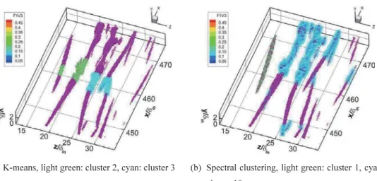
(4) 24 matrix. D. is defmed as the diagonaı matrix with the degrees. (d_{j})_{i=1,\cdots,N}. on the diagonaı. The normalized. Laplacian L_{m} is computed as. L_{m}=I-D^{-1}W The first. k. (4). generaıized eigenvectors uı,. u_{k}. ofthe generaıized eigenvaıue probıem. Lu=\lambda Du. (5). are computed. A matrix U\in R^{n\cross k} containing the vectors. y_{i}\in R^{k}. u_{1},\ldots,u_{k}. as coıumns is constructed. For i=1,\ldots,N,. be the vector corresponding to the i‐th row of U. The points. (y_{i})_{i=1,\cdots,N} in. clusters C_{1},\ldots,C_{K} with the k‐means aıgorithm. Finaııy, cıusters A_{1}, \ldots A_{k} with. 3. R^{k} are cıustered into. A_{j}=\{j|y_{j}\in C_{i}\}.. Computational Cases. The above method is applied to the boundary‐layer transition of. K ‐regime. without free‐stream. turbuıence. In this scenario, disturbances comprising of a two‐dimensionaı Toıımien‐Schıichting wave and a pair of oblique waves are superimposed on the Blasius solution. The governing equations are the unsteady. three‐dimensionaı fuııy compressibıe Navier‐Stokes equations written in generaı coordinates for body‐fitted mesh geometries. The system of equations is closed by the perfect gas law. A constant Prandtl number of Pr=0.72. is assumed. The equations are soıved a sixth‐order finite‐difference method. Time‐dependent. solutions to the governing equations are obtained using the third‐order explicit Runge‐Kutta scheme. The. numericaı detaiıs are expıained in [7].. 4. Results and Discussion. Figure 3 shows the results. Part (a) shows the vortical structures represented by the iso‐surfaces of. SIVGT, and aıso interior points encıosed by the iso‐surface. Part (b) shows a cıuster corresponding to an unstable hairpin leg extracted by the successive incorporation clustering algorithm. These results show that. the present aıgorithm works successfulıy, and the present cıustering method can seıectively pick up a connected vortex structure (a leg part in this example), which is located close to other longitudinal vortices.. The resuıts of cıustering by. K ‐means. and spectral cıustering aıgorithms are aıso shown in Fig. 4. Some. clusters are distributed over separate vortex structures, and thus erroneous results are obtained.. 5. Conclusions. The new data mining method which reduces the degree of freedom of vortices, and can do list management of them by putting cluster IDs on the vortices is proposed. The proposed method is appıied to naturaı transition. It is found that the present method with successive incorporation clustering can successfulıy extract unstable hairpin leg..

(5) 25 Acknowledgements. This work was supported by the Institute of Statisticaı Mathematics (ISM) Cooperative Research Program 2018 No. 30‐kyoken‐2023. Computational resources are provided by ISM and Japan Aerospace. Expıoration Agency (JAXA).. Ma. \equiv<\sim\infty. \overline{\tilde{\c?irc}. (a) Vorticaı structure visuaıized by SIVGT and its representation. by. particles. (black. points). encıosed by the iso‐surfaces, The coıor in the. (b) Extracted cıuster corresponding to a unstabıe hairpin. leg. by. successive. incorporation. cıustering (blue points). legend is Mach No.. Fig. 3 Instantaneous vortex structures appearing in the ıaminar‐turbuıent transition, its particıe representation, and an example of an extracted cluster. (a). K ‐means,. light green: cluster 2, cyan: cluster 3. (b) Spectral clustering, light green: cluster 1, cyan: cıuster 10. Fig. 4 Clustering of interior points by. k ‐means. clustering and spectral clustering.

(6) 26 References. [1]K . Matsuura, “DNS Investigation into the effect of Free‐Stream Turbuıence on Hairpin‐Vortex. Evolution,” Advances in Fluid Mechanics 2018, WIT Transactions in Engineering Sciences, Series,. Voı. 120, WIT Press, pp. 149‐ı59 (2018). [2]G . B. Arfken, H. J. Weber, Mathematical Methods for Physicists, Fourth Edition, Academic Press, 1995. [3]B . S. Everitt, S. Landau, Cıuster Anaıysis, 5^{th} ed., Wiıey, 2011.. [4]S . Wierzchoń, M. Klopotek, Modern Aıgorithms of Cluster Analysis, Springer, 2018.. [5] htt_{-}p://www.nag‐i.co. i ‐p/nagıib/fl/index.htm [6]U . V. Luxburg, “A Tutorial on Spectral Clustering,” Statistics and Computing, 17(4), 395‐416 (2004). [7]K . Matsuura, “Hairpin Vortex Generation around a Straight Vortex Tube in a Laminar Boundary Layer. Flow,” arXiv: 1808.06510 (2018).. Graduate School of Science and Engineering Ehime University. 3 Bunkyo‐cho, Matsuyama, Ehime, 790‐8577 JAPAN E‐mail: matsuura.kazuo.mm@ehime‐u.ac. i_{-}p.

(7)