Spreading profiles of solutions to a free boundary problem for a reaction-diffusion equation (Qualitative Theory on ODEs and their applications to Mathematical Modeling)

全文

(1)9. Spreading profiles of solutions to a free boundary problem for a reaction‐diffusion equation* 早稲田大学基幹理工学部数学科兼子裕大. Department of Pure and Applied Mathematics, Waseda University Yuki Kaneko†. 1. Introduction In this article we will discuss some recent results by Kaneko‐Matsuzawa‐. Yamada [11] on a free boundary problem for a reaction‐difFusion equation. We consider a free boundary problem for a reaction‐diffusion equation given by. where. \mu. \begin{ar y}{l u_{t}=u_{x}+f(u), t>0,<xh(t), u_{x}(t,0)=,u(th )=0, t>0, h'(t)=-\mu _{x}(t,h ) , t>0, h(0)=h_{0},u(0,x)=u_{0}(x), 0\leqx\leqh_{0}, \end{ar y}. and h_{0} are positive constants, and the initial function. u_{0}\in C^{2}([0, h_{0}]) ,. u_{0}>0. in [0, h_{0}) ,. u_{0}. (1.1). satisfies. u_{0}'(0)=u_{0}(h_{0})=0 and u_{0}'(h_{0})<0.. Moreover nonlinear function f(u) is assumed to satisfy the following conditions:. \begin{ar y}{l f(u)=0ifandonlyifu=0,u_{1}^*,u_{2}^*,u_{3}^* with0<u_{1}^* <u_{2}^*<u_{3}^*, f'(0)> ,f'(u_{1}^*)<0,f'(u_{2}^*)>0,f'(u_{3}^*)<0and \int_{u 1}^{* u_{3}^* f(u)d >0. \end{ar y}. (1.2). The nonlinear term is called positive bistable nonlinearity. Different from the typical bistable nonlinearity, it has two positive stable equilibrium states u_{1}^{*}, u_{3}^{*}.. Problem (1.1) may be applied to model the spreading of new or inva‐ sive species in ecology.. The spread of biological species is one of the cen‐. tral topic in mathematical ecology. Since Skellam’s investigation (Skellam [18]), invasion phenomena have been widely studied by lots of researchers (see e.g . Shigesada‐Kawasaki [17]). Nonlinearity (1.2) was especially introduced by Ludwig‐Aronson‐Weinberger [15] to model the population dynamics of spruce This article was based on the joint work with Professor Hiroshi Matsuzawa (National Institute of Technology, Numazu College) and Professor Yoshio Yamada (Waseda Univeristy) *. \dagger The author was partially supported by Waseda University Grant for Special Research. Projects (2018K‐203, 2018B‐l03)..

(2) 10 budworm in North America. The difference between previous works on in‐. vasion phenomena and problem (1.1) is that the problem is described as a free boundary problem, where u(t, x) represents the population density of a species and free boundary h(t) denotes the spreading front of one‐dimensional habitat (0, h(t)) . The dynamical behavior of the free boundary is also deter‐ mined by Stefan condition h'(t)=-\mu u_{x}(t, h(t)) . We consider a pair of solution (u(t, x), h(t)) to (1.1) to investigate the spread of new or invasive species. This type of free boundary problem was first proposed by Du‐Lin [2] when f(u)=u(a-bu) for a, b>0 . They obtained the existence and uniqueness of global solutions and showed spreading and vanishing in large time behaviors. of solutions. For any solution of their free boundary problem, either (i) or (ii) holds as tarrow\infty :. \lim_{tar ow\infty}u(t, x)=\frac{a}{b} locally uniformly in \mathbb{R}, Vanishing: t ar ow\infty 1\dot{ \imath} mh(t)\leq\frac{\pi}{2\sqrt{a} and \lim_{tar ow\infty}\sup_{0\leq x\leq h(t)}|u(t, x)|=0.. (i) Spreading: (ii). \lim_{tarrow\infty}h(t)=\infty. and. After the work of Du‐Lin [2], their results were extended by many researchers (cf. [3]-[4], [6]-[14] ). We also refer to Mimura‐Yamada‐Yotsutani [16] a free boundary problem for a system of reaction‐diffusion equations. It is seen that. problem (1.1) has a unique classical solution (u(t, x), h(t)) satisfying 0<u(t, x)\leq C_{1}. for. t>0,0<x<h(t). and. 0<h'(t)\leq\mu C_{2}. for. t>0. for some constants C_{1}, C_{2}>0 when f is locally Lipschitz continuous in [0 , oo), f(0)=0 and f(u)<0 for all large u>0 (see Kaneko‐Yamada [9]). Moreover Kawai‐Yamada [12] studied problem (1.1) with positive bistable nonlinearity (1.2). They showed that exactly one of the followings occurs for any solution (u, h) as tarrow\infty : (i) Vanishing:. \lim_{tar ow\infty}h(t)\leq\frac{\pi}{2\sqrt{f'(0)}. and. \lim_{tar ow\infty}\sup_{0\leq x\leq h(t)}|u(t, x)|=0,. (ii) Small Spreading: (iii). (iv). \lim_{tarrow\infty}h(t)=\infty and \lim_{tarrow\infty}u(t, x)=u_{1}^{*} locally uniformly in \mathbb{R}, Big Spreading: \lim_{tarrow\infty}h(t)=\infty and \lim_{tarrow\infty}u(t, x)=u_{3}^{*} locally uniformly in \mathbb{R}, Transition : \lim_{tarrow\infty}h(t)=\infty and \lim_{tarrow\infty}u(t, x)=V(x) locally uniformly in \mathbb{R}, where V(x) is a unique solution to. V"+f(V)=0. in. (0, \infty), V'(0)=0. and. \lim_{xarrow\infty}V(x)=u_{1}^{*}.. The main purpose of this article is to show the asymptotic profile of solu‐ tions as tarrow\infty . Since small and big spreading mean local uniform convergence. of u(t, \cdot) in. \mathbb{R}. (that is, uniform convergence in [0, R] for any. R>0 ),. they do.

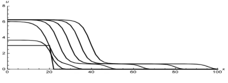
(3) 11 11. not give detailed information near the free boundary. It is known that, for typical type of f , the spreading speed and the asymptotic profiles of solutions near the spreading front are determined by the following semi‐wave problem:. (SWP). \{\begin{ar ay}{l} q" - cq'+f(q)=0, q(z)>0 for z>0, q(0)=0, \mu q'(0)=c,\lim_{zar ow\infty}q(z)=u^{*}, \end{ar ay}. where \mu is given in (1.1) and u^{*} stands for a positive zero point of f . For solution (c^{*}, q^{*}) to (SWP), we call function q^{*} semi‐wave and refer to c^{*} as spreading speed. When u^{*}=u_{1}^{*} (corresponding to the small spreading case), there exist a unique solution pair (c, q)=(c_{S}, q_{S}) to (SWP) and a constant H ム \in \mathbb{R} such that. tarrow\infty 1\dot{{\imath}}m(h(t)-c_{S}t)=Hム. and. \lim_{tarrow\infty}\sup_{0\leq x\leq h(t)}|u(t, x)-qs(h(t)-x)|=0.. However the situation for u^{*}=u_{3}^{*} (the big spreading case) is more complicated and it is divided into two cases: (Case A) there exists a a unique solution pair to (SWP) for any \mu>0 , while (Case B) we can find some \mu^{*}>0 such that (SWP) has a unique solution pair (c_{B}, q_{B}) to (SWP) for \mu<\mu^{*} and no solutions for \mu\geq\mu^{*} . Moreover average speed is given by. \lim_{tarow\infty}\frac{h(t)}{t=\{ begin{aray}{l c_{B}, if\mu<\mu^{*}, c_{S}, if\mu\geq\mu^{*}. \end{aray}. If (SWP) with u^{*}=u_{3}^{*} has a unique solution, it is possible to show that the asymptotic profile of that is,. u. near the free boundary is determined by the semi‐wave,. \lim_{tarrow\infty}(h(t)-c_{B}t)=H^{*}. and. \lim_{tarrow\infty}\sup_{0\leq x\leq h(t)}|u(t, x)-q_{B}(h(t)-x)|=0. for some constant H^{*}\in \mathbb{R} . In the other case the asymptotic profile of solutions is not obtained by (SWP) with u^{*}=u_{3}^{*} . Then it was numerically observed. that the solution to (1.1) can form a so called propagating terrace (see Figure 1). The notion of propagating terrace arise from Ducrot‐Giletti‐Matano [5] for a Cauchy problem of a reaction‐diffusion equation. We are thus interested in such a terraced profile of solutions.. Figure 1 : Numerical example for terraced profile.

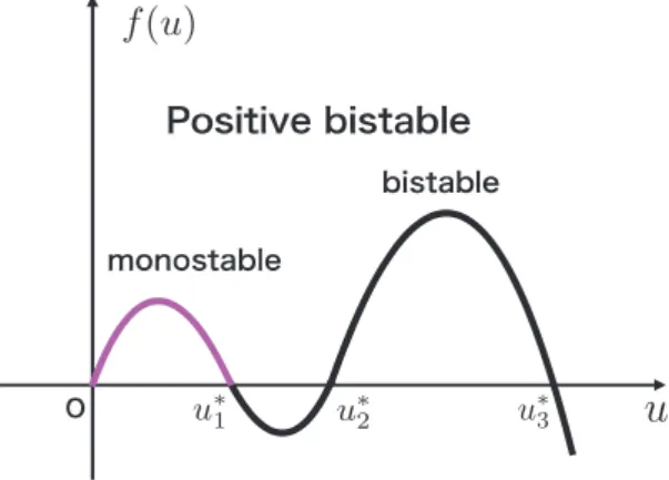
(4) 12 This article is organized as follows: in Section 2 we prepare some notations and an assumption. Section 3 is devoted to main results concerning on the profile of propagating terrace and the proofs of the main results.. 2. Notations and assumption (TW) In this section we will prepare for main results. Let c_{S}(\mu) and c_{B}(\mu) be. defined as in Section 1. Here. \mu. is a given constant in (1.1) and we make it. clear the dependence of the spreading speeds on \mu. We now prepare traveling waves to explain the relation with c_{S}(\mu) and c_{B}(\mu) . One can regard positive bistable term f(u) as the combination of f|_{[0,u_{1}^{*}]} and f|_{[u_{2}^{*},u_{3}^{*}]} , where f|_{[a,b]} denotes the restriction of f onto [a, b] . Then. we see f|_{[0,u_{1}^{*}]} as monostable term and f|_{[u_{2}^{*},u_{3}^{*}]} as bistable one (see Figure 2), and get a traveling wave corresponding to each part in the following way.. Figure 2 : Positive bistable term Consider. \{ begin{ar ay}{l Q"-cQ'+f(Q)=0,q(z)>0for-\infty<z<\infty, \lim_{zar ow-\infty}Q(z)=u_{1}^{*},Q(0)=(u_{1}^{*}+u_{3}^{*})/2, \lim_{zar ow\infty}Q(z)=u_{3}^{*} \end{ar ay}. (2.1). \{\begin{ar ay}{l} Q"-cQ'+f(Q)=0, q(z)>0 for -\infty<z< o , \lim_{zar ow-\infty}Q(z)=0, Q(0)=u_{1}^{*}/2,\lim_{zar ow\infty}Q(z)=u_{1}^{*}. \end{ar ay}. (2.2). and. It is well known that there exists a unique c=c_{1}^{B} such that (2.1) has a unique (up to shift) solution Q=Q_{1}^{B}(z) and that (2.2) has solutions for |c|\geq c_{0}^{S} for a minimal speed. c_{0}^{S}>0..

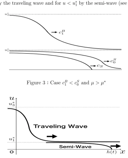
(5) 13 To get the terraced profile we need an assumption. Recall Case B in Section 1; where (SWP) with u^{*}=u_{3}^{*} has no solutions for large \mu . Then \lim_{tarrow\infty}h(t)/t=c_{S} . It is necessary to assume c_{1}^{B}<c_{0}^{S} to deduce this esti‐. mate. By Kawai‐Yamada [12] and Du‐Lou [3], we find that semi‐wave speeds c_{S}(\mu), c_{B}(\mu) are increasing with respect to \mu , and satisfy. c_{S}(\mu)<c_{0}^{S}, c_{B}(\mu)<c_{1}^{B} and. c_{S}(\mu)arrow c_{0}^{S} assume c_{1}^{B}<c_{0}^{S} , then as. If we. \muarrow\infty,. c_{S}(\mu)arrow 0. as. \muarrow 0.. there exists \mu^{*}>0 such that. c_{S}(\mu^{*})=c_{1}^{B} , and. hence c_{S}(\mu)>c_{1}^{B} for \mu>\mu^{*} (see Figure 3). In the rest of the article we assume (TW). c_{1}^{B}<c_{0}^{S} and. \mu>\mu^{*}.. Our strategy to get the terraced profile is to approximate the solution for u\geq u_{1}^{*} by the traveling wave and for u<u_{1}^{*} by the semi‐wave (see Figure 4).. Figure 3 : Case. c_{1}^{B}<c_{0}^{S} and. \mu>\mu^{*}. Figure 4: Approximation by traveling wave and semi‐wave.

(6) 14 Finally we prepare a comparison principle which is useful to prove main results. A pair of functions (\underline{u}, \underline{h}) in the following lemma is called lower solution. to (1.1). An upper solution is defined in a similar way.. \underline{h}\in C^{1}([0, T]) and \underline{u}\in C(\Omega_{1})\cap C^{1,2}(\Omega_{1}) \mathbb{R}^{2}|0\leq x\leq\underline{h}(t) for 0<t\leq T } satisfy. Lemma 1. Let. with. \Omega_{1}=\{(t, x)\in. \{begin{ar y}{l \underli {u}_t\lequnderli {u}_x+f(\underli {u}),(tx)\inOmega_{1} , \underli {u}_x(t,0)\geq0,\underli {u}(t,\nderli {h}(t)=0,t\in(0, T] \underli {h}'(t)\leq-mu\nderli {u}_x(t,\underli {h}(t), \in(0,T]. \end{ar y} If \underline{h}(0)\leq h_{0} and \underline{u}(0, x)\leq u_{0}(x) in [0, \underline{h}(0)] , then. \underline{h}(t)\leq h(t). 3. in. [0, T]. and. \underline{u}(t, x)\leq u(t, x). in. \overline{\Omega}_{1}.. Main results and proofs. 3.1. Main results. We will see main results in this section. Let (u, h) be a solution to (1.1). We call (u, h) big spreading solution if and only if u(t, x) and h(t) satisfy. \lim_{tarrow\infty}h(t)=\infty. and. \lim_{tarrow\infty}u(t, x)=u_{3}^{*}. locally uniformly in. \mathbb{R}.. The following result is concerned with rough estimates of the asymptotic profile of solutions.. Theorem 1 ([11]). Assume (TW). Let (u, h) be any big spreading solution to (1.1). For any small \varepsilon>0 , there exist M>0, \delta>0 and T>0 such that for t\geq T. \sup_{x\in[0,(c_{1}^{B}-\varepsilon)t]}|u(t, x)-u_{3}^{*}|\leq Me^{-\delta t} , \sup_{x\in[(c_{1}^{B}+\varepsilon)t,(c_{S}-\varepsilon)t]}|u(t, x)-u_{1}^{*} |\leq Me^{-\delta t} , where c_{1}^{B} denotes the speed of traveling wave defined in Section 2 and resents the speed of semi‐wave defined in Section 1.. (3.1) (3.2) c_{S}. We will explain a terraced profile of big spreading solutions to (1.1).. rep‐.

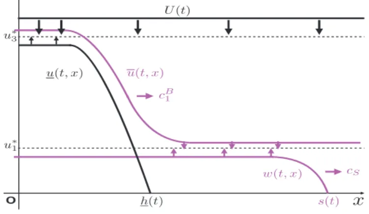
(7) 15 Theorem 2 ([11]). Assume (TW). Let (u, h) be any big spreading solution to (1.1) and let (c_{S}, q_{S}) be the solution to (SWP) with u=u_{1}^{*} . Then, for any. c\in(c_{1}^{B}, c_{S}) , there exist H_{S},. H_{B}\in \mathbb{R} such that. \lim_{tarrow\infty}(h(t)-c_{S}t-H_{S})=0, \lim_{tarrow\infty}h'(t)=c_{S},. \lim_{tarrow\infty}\sup_{x\in[ct,h(t)]}|u(t, x)-q_{S}(h(t)-x)|=0. and. \lim_{tarrow\infty}\sup_{x\in[0,ct]}|u(t, x)-Q_{1}^{B}(c_{1}^{B}t+H_{B}-x)|=0, where Q_{1}^{B} is a unique solution to (2.1) with c=c_{1}^{B}. 3.2. Proof of Theorem 1. We first show (3.1). Let U=U(t) be a solution of. \{ begin{ar ay}{l U_{t}=f(U),t>0, U(0)=a>\max\{ Vertu_{0}\Vert_{C([0,h_{0}])},u_{3}^{*}\ . \end{ar ay} Then the standard comparison principle gives u(t, x)\leq U(t) for t>0,0<x< h(t) . Moreover U(t) is monotone decreasing with respect to t and converges to u_{3}^{*} as tarrow\infty . From the linearization problem at U=u_{3}^{*} , we can choose positive constants T^{*}, \delta and M such that. u(t, x)\leq u_{3}^{*}+Me^{-\delta t} c\in(0, c_{1}^{B}) .. for. t\geq T^{*}, 0\leq x\leq h(t) .. q_{c}=q_{c}(z) be a solution of q_{c}"-cq_{c}'+f(q_{c})=0 such that Q_{c} :=q_{c}(0)<u_{3}^{*}, q_{c}'(0)=0, q_{c}(-z_{1})=0 and q_{c}'>0 in [-z_{1},0) for some constant z_{1}>0 . Then we see Q_{c}arrow u_{3}^{*} as carrow c_{1}^{B} . Define Fix. Let. \underline{u}(t, x)=\{\begin{ar ay}{l } Q_{c}, 0\leq x\leq ct, q_{c}(ct-x) , ct\leq x\leq ct+z_{1} \end{ar ay} Letting. c. \underline{h}(t)=ct+z_{1}.. and. sufficiently close to c_{1}^{B} , we deduce from Lemma 1 that. \underline{h}(t-T_{1})\leq h(t). for. t\geq T_{2},. \underline{u}(t-T_{1}, x)\leq u(t, x). for. t>T_{2},0\leq x\leq\underline{h}(t-T_{1}). for some constants T_{1}, T_{2} with T_{1}<T_{2} . In particular u(t, x)\geq Q_{c} for t\geq T_{2},0\leq x\leq c(t-T_{1}) . Moreover, taking c(<c_{1}^{B}) and T^{*} suitably large, we have. (c_{1}^{B}-\varepsilon)t\leq c(t-T_{1}). for. t\geq T^{*}. Using the above estimate and Q_{c}arrow u_{3}^{*} as carrow c_{1}^{B} , one can choose suitable constant T^{*}, M, \delta>0 satisfying. u(t, x)\geq u_{3}^{*}-Me^{-\delta}オ. f。r. t\geq T^{*},. 0\leq x\leq(c_{1}^{B}-\varepsilon)t..

(8) 16 These estimates show (3.1) (See Figure 5). We next prove (3.2). It is easy to check that. s(t)=c_{S}(t-T)+h_{0}, w(t, x)=q_{S}(s(t)-x) is a lower solution to (1.1) for t\geq T, 0\leq x\leq s(t) . Note that there exist C_{0}, \gamma>0 satisfying q_{S}(z)\geq u_{1}^{*}-C_{0}e^{-\gamma z} for z\geq 0 . Then, for any c\in(0, c_{S}) , we obtain. u(t, x)\geq u_{1}^{*}-\tilde{M}e^{-\overline{6}t} t\geq\tilde{T}, 0\leq x\leq ct with some constants. \tilde{T},\tilde{M},\tilde{\delta}>0 .. Let. \overline{u}(t, x)=Q_{1}^{B}(c_{1}^{B}(t-T_{0})+X_{0}+M_{0}\rho(e^{-\delta_{0} T_{0}}-e^{-\delta_{0}t})-x)+M_{0}e^{-\delta_{0}t} for positive constants T_{0}, X_{0}, M_{0}, \rho and \delta_{0} . Then, by choosing the constants suitablely, the standard comparison principle proves u(t, x)\leq\overline{u}(t, x) for t\geq T_{0}, 0\leq x\leq h(t) . This estimate enables us to get, for any c\in(c_{1}^{B}, c_{S}). u(t, x)\leq u_{1}^{*}+M_{0}e^{-\delta_{0}t} t\geq T_{0}, ct\leq x\leq h(t) by adjusting the constants (see Figure 5). These estimates prove (3.2).. 口. Figure 5 : Functions compared with solutions 3.3. Proof of Theorem 2. The spreading speed estimate and the convergence of. u. to semi‐wave. q_{S}. are. proved by a similar manner as in Du‐Matsuzawa‐Zhou [4] and Kaneko‐Yamada [10] by zero number arguments and the comparison principle. Hence it remains. to show the convergence to traveling wave Q_{1}^{B} . As in the proof of Theorem 1, we can construct upper and lower solutions and find some constants H_{0}, H_{1}\in \mathbb{R} and T, M, \delta>0 such that. Q_{1}^{B}(c_{1}^{B}t+H_{1}-x)-Me^{-\delta t}\leq u(t, x)\leq Q_{1}^{B}(c_{1} ^{B}t+H_{0}-x)+Me^{-\delta t}.

(9) 17 for. t\geq T, 0\leq x\leq ct with. c\in(c_{1}^{B}, c_{S}) .. Define. v(t, z)=u(t, z+c_{1}^{B}t) .. Then it. follows that. Q_{1}^{B}(H_{1}-z)-Me^{-\delta t}\leq v(t, z)\leq Q_{1}^{B}(H_{0}-z)+Me^{- \delta t} for t\geq T, -c_{1}^{B}t\leq z\leq(c-c_{1}^{B})t . By Berestycki‐Hamel [1], v(t, z) converges along subsequences \{t_{n}\} to a traveling waves locally uniformly in \mathbb{R} , that is,. v(t_{n}, z)arrow Q_{1}^{B} (HB—Z) locally uniformly in. \mathbb{R}. as. narrow\infty. for some constant H_{B} . We can finally prove that H_{B} does not depend on the subsequences by constructing appropriate upper and lower solutions. The proof is complete. 口. Acknowledgements The author would like to thank organizers, especially Professor Tohru Wakasa, for giving him the opportunity to present the study in RIMS Work‐ shop.. References [1] H. Barestycki and F. Hamel, Generalized traveling waves for reaction‐ diffusion equations, in “Perspective in Nonlinear Partial Differential Equa‐ tions in honor of H. Brezis, Contemp. Math., Vol. 446, Amer. Math. Soc., Providence, RI, 2007, pp. 211‐237.. [2] Y. Du and Z. G. Lin, Spreading‐vanishing dichotomy in the diffusive l0‐ gistic model with a free boundary, SIAM J. Math. Anal., 42 (2010), pp. 377‐405.. [3] Y. Du and B. Lou, Spreading and vanishing in nonlinear diffusion prob‐ lems with free boundaries, J. Eur. Math. Soc., 17 (2015), pp. 2673‐2724. [4] Y. Du, H. Matsuzawa and M. Zhou, Sharp estimate of the spreading speed determined by nonlinear free boundary problems, SIAM J. Math. Anal.,. 46 (2014), pp. 375‐396.. [5] A. Ducrot, T. Giletti and H. Matano, Existence and convergence to a prop‐ agating terrace in one‐dimensional reaction‐diffusion equations, Trans.. Amer. Math. Soc., 366 (2014), pp. 5541‐5566. [6] J. S. Guo and C. H. Wu, Dynamics for a two‐species competition‐diffusion model with two free boundaries, Nonlinearity, 28 (2015), pp. 1‐27..

(10) 18 [7] J. S. Guo and C. H. Wu, On a free boundary problem for a two‐species weak competition system, J. Dyn. Diff. Equat., 22 (2012), pp. 873‐895. [8] Y. Kaneko, K. Oeda and Y. Yamada, Remarks on spreading and vanishing for free boundary problems of some reaction‐diffusion equations, Funkcial.. Ekvac., 57 (2014), pp. 449‐465. [9] Y. Kaneko and Y. Yamada, A free boundary problem for a reaction‐ diffusion equation appearing in ecology, Adv. Math. Sci. Appl., 21 (2011), pp. 467‐492.. [10] Y. Kaneko and Y. Yamada, Spreading speed and profiles of solutions to a free boundary problem with Dirichlet boundary conditions, J. Math. Anal.. Appl., 465 (2018), pp. 1159‐1175. [11] Y. Kaneko, H. Matsuzawa and Y. Yamada, Asymptotic profiles of solu‐ tions and propagating terrace for a free boundary problem of nonlinear diffusion equation with positive bistable nonlinearity, preprint.. [12] Y. Kawai and Y. Yamada, Multiple spreading phenomena for a free bound‐ ary problem of a reaction‐diffusion equation with a certain class of. bi_{\mathcal{S}}table. nonlinearity, J. Differential Equations, 261 (2016), pp. 538‐572. [13] X. Liu and B. Lou, Asymptotic behavior of solutions to diffusion problems with robin and free boundary conditions, Math. Model. Nat. Phenom., 8. (2013), pp. 18‐32. [14] X. Liu and B. Lou, On a reation‐diffusion equation with Robin and free boundary conditions, J. Differential Equations, 259 (2015), 423‐453.. [15] D. Ludwig, D.G. Aronson and H.F. Weinberger, Spatial patterning of the spruce budworm, J. Math. Biol., 8 (1979), pp. 217‐258. [16] M. Mimura, Y. Yamada and S. Yotsutani, A free boundary problem in ecology, Japan J. Appl. Math., 2 (1985), pp. 151‐186. [17] N. Shigesada and K. Kawasaki, Biological invasions: Theory and Practice, Oxford Series in Ecology and Evolution, Oxford Univ. Press, 1997.. [18] J. G. Skellam, Random dispersal in theoretical populations, Biometrika, 38 (1951), pp. 196‐218..

(11)