1oe
A Robust
Boosting
Method
using
ZerO-0ne Loss
Function
:
SNRBoost
筑波大学大学院 社会工学研究科 佐野 夏樹(Natsuki Sano)
The Doctoral Program in Policy and Planning Sciences
University of Tsukuba
筑波大学・社会工学系 鈴木 秀男 (Hideo Suzuki)
Institute of Policy and Planning Sciences
University ofTsukuba
筑波大学 $\urcorner$
社会工学系 香田 正人(Masato Koda)
Institute ofPolicy and Planning Sciences
University of Tsukuba
Abstract
We propose anew, robust boostingmethod by usingazer0-0ne step
func-tionas aloss function. In deriving the method, the margin boost technique is
blended with the derivative approximation algorithm, called Stochastic Noise
Reaction (SNR). Basedon intensivenumerical experiments, we show that the
proposed method is actually betterthan other boosting methodson testerror
rates in the case of noisy, mislabeled situation.
Key words: AdaBoost, MarginBoost, ZerO-0ne Loss Function, Stochastic Noise
Reaction.
1.
Introduction-AdaBoost
Supposeasituation in whichamanagement must solve a decision problem depending
on a number of people whose opinions differ slightly, and their experiences and
personal abilities to solve the problem seem to be almost equal and, as a result,
cannot draw a decisive conclusion. To resolve this situation in order to make a
reasonably better decision, is it more efficient to ignoreopinions of these people and
relying solely on manager’s decision, or to restart the discussion by changing the
team and forming a new ensemble through addition of capable people?
Obviously, the first behaviour is faster but it may not lead to a better decision.
On theotherhand, the second one maylead to abetter decisionsinceit willprovide
an iterative improvement to the solution but it certainly is a slow process and
takes much longer time. This is what we often encounter during decision analysis
dealing with data mining. However, we can make a better decision even in the
originalsituation by resortingto theiterativeimprovement method considering that
a possible better solution is still the outcome of a combination of a set of slightly
different opinions converging toward the genuine better one.
Thesituation described above isessentiallyaproblemassociated with a committee
based decision making. The aimof this paper is to develop anew robust algorithm
for pattern classification problem by using an analogy to the committee-based
de-cision making, where each individual member of the committee corresponds to a
classifier. The decision here is to correctly classify data to its true class label, and
we would like to develop a new robust classification method through iterative
im-provement of classifiers or committee members.
In view of the above objective in mind, the starting point for the present study
would be an iterativeimprovement procedure called boosting, whichis awayof
com-bining the performance ofmany weak classifiers to produce a powerful committee.
The procedure allows the designer to continue adding weak classifiers until some
desired low training error has been achieved. Boostingtechniques have mostly been
studied in the computational learning theory literature (e.g., see Schapire (1990),
Freund (1995), Freund and Schapire (1997)$)$ and received increasing attention in
many areas including data mining and knowledge discovery.
While boosting has evolved over the recent years, we focus on the most
com-monly used version of the adaptiveboosting procedure, i.e., “
AdaBoost.Ml. ”
(Fre-und and Schapire, 1997). A concise description of AdaBoost is given here for
the tw0-category classification setting. We have a set of $n$ trainning data pairs,
$(x_{1}, y_{1})$,$\ldots$,$(x:, y:)$,
.
. .
’$(x_{n}, y_{n})$, where $x$: denotes a vector valued feature with $y_{i}=$
$-1$ or 1, as its class label or teacher signal. The total number of component
classi-fiers is assumed to be $T\mathrm{r}$ Then, the output ofclassification model (i.e., committee)
is given by a scalar function, $F(x)= \sum_{t=1}^{T}\beta_{t}f_{t}(x)$, in which each $\mathrm{f}_{t}(x)$ denotes a
classifier producing values +1, and $\beta_{t}$ are prescribed constants; the corresponding
prediction (i.e., decision) is sign(F(x)).
The AdaBoost procedure trains the classifiers $f_{t}(x)$ on weighted versions of the
training sample, by giving higher weight to cases that are currently misclassified.
This isdonefor asequenceof weightedsamples, and thenthefinal classifier is defined
to be a linear superposition ofthe classifiers fromeach stage. A detailed desciption
of AdaBoost.Ml. is summarized and given in the next box, where $I(y:\neq f_{t}(x_{i}))$
denotes the indicator function with respect to the event such that $y:\neq 7t$($\mathrm{x}\mathrm{n}$, i.e.,
misclassification event.
At $t$-th iteration stage, given the observation weight $ce_{t-1}(i)$, AdaBoost fits a
classifier $f_{i}(x)$ to the training data $Xj$ $(i=1,2, \ldots,n)$ that is weighted by $w_{t-1}(i)$
.
Then, it evaluates the weighted error $\mathrm{e}\mathrm{r}\mathrm{r}_{\mathrm{t}}$ by computing a weighted count of
mis-classification events as $\mathrm{e}\mathrm{r}\mathrm{r}_{t}=$
Er
$=1w_{t-1}(i)I(y:\neq f_{t}(x:))$.
Using $\mathrm{e}\mathrm{r}\mathrm{r}_{t}$, $\beta_{t}$ is obtained as $\beta_{t}=\log$((1 –errt)/errt). Finally, the observation weight is updated throughthe computation of $w_{t}(i)=w_{t-1}(i)\exp[\mathcal{B}_{t}I(y:\neq f_{t}(x:))]$ aad normalized so that
$\sum_{=1}^{n}.\cdot w_{t}(i)=1.$ This results in giving a heigher weight to the training data that is
currently misclassified.
Much has been written about the success of AdaBoost in producing accurate
classifiers. Many authors have explored the use of a tree based classifier for $f_{t}$(x)
and demonstrated that it consistently produces significantly lower error rates than
a single decision tree. In fact, Breiman called
Ada,B,
oost with trees as “the best
108
AdaBoost.Ml. (Freund and Schapire, 1997)
1. Initialize the observation weights $wo(i)=1/n$ for $i=1,$2,$\ldots$ ,$n$,
and $F_{0}(x)=0.$
2. For $t=1,2$,$\ldots$ ,$T$ do
(a) Fit a classifier $f_{t}(x)$ to the training data weighted by $\mathrm{p}_{1-1}(\mathrm{j})$
.
(b) Compute $\mathrm{e}\mathrm{r}\mathrm{r}_{t}=\sum_{i=1}^{n}w_{t-1}(i)I(yj\neq f_{t}(x.\cdot))$.
(c) Compute $\beta_{t}=\log((1-\mathrm{e}\mathrm{r}\mathrm{r}_{t})/(\mathrm{e}\mathrm{r}\mathrm{r}_{t}))$
.
(d) Let $F_{t}(x)=F_{t-1}(x)+\beta_{t}f_{t}(x)$
.
(e) Set $w_{t}(i)=w_{t-1}(i)\exp[\beta_{t}I(y\dot{.}\neq f_{t}(x_{i}))]$, and normalize $\mathrm{w}\mathrm{t}(\mathrm{i})$
so that $\sum_{=1}^{n}\dot{.}w_{t}(i)=1$ for $i=1,2$,$\ldots$,$n$
.
end For
3. Output sign(F\mbox{\boldmath $\tau$}(x)).
Interestingly, in many examples, the test error seems to consistently decrease
and then level off as
more
classifiers are added, instead of turning into ultimateincrease. It hence seems that AdaBoost is resistent to overfitting for low noise
cases. However, recent studies with highly noisy patterns (Quinlan, 1996; Grove
and Schuurmans, 1998; Ratsch et al., 1998) depict that it is clearly a myth that
AdaBoost do not overfit sinceAdaBoost asymptoticallyconcentrateon the patterns
which are hardest to learn. To cope with this problem, some regularized boosting
algorithms (Mason et al., 1999; Ritsch et al., 1998) are proposed. In this paper, we
$\mathrm{w}\mathrm{i}\mathbb{I}$take an iterative improvement approach to optimize classifiers to derive a new
robust boosting method that is resistent against mislabeled noisy patterns.
In the next section, we present the principles of MarginBoost. We also roughly
explain an outline of LogitBoost in Section 2. Then, in Section 3, we present the
zer0-0nelossfunction and StochasticNoiseReaction (SNR). InSection4,we propose
the new robust boosting method and results ofintensive numerical experiments
are
presented, and we detail cases with noisy, mislabeled patterns. Section 5 contains
some concluding remarks.
2.
Margin Boost
We assumethat the training data set $(x,y)$ israndomlygenerated accordingto some
unknownprobabilitydistribution Z) on$X\mathrm{x}Y$ where$X$isthe space ofmeasurements
(typically $X\subseteq \mathbb{R}^{N}$) and $\mathrm{Y}$ is the space of labels ($\mathrm{Y}$ is usually a discrete set or some
given by
$F(x)= \sum_{t=1}^{T}\beta_{t}f_{\mathrm{t}}(x)$, (1)
and $f_{t}(x)$ : $Xarrow\{\pm 1\}$ are base classifiers from some fixed class $\mathrm{i}$, and
$\beta_{t}\in \mathbb{R}$
denotes theclassifier weights. The margin of the training data $(x, y)$ with respect to
the classifier, i.e., sign(F(x)), is defined as $yF(x)$
.
It is notedthat if$y\neq$ sign(F(s))then $yF(x)<0,$ and if$y=\mathrm{s}\mathrm{i}\mathrm{g}\mathrm{n}(F(x))$ then $yF(x)\geq 0.$ Margin can be understood
as a mesure of difficulty of classification. As data has a larger (positive) margin,
the example is easier to classify. On the contrary, as it has a smaller (negative)
margin, the data is harder to classify. Given a set $S=\{(x_{1}, y_{1}), \ldots, (x_{n}, y_{n})\}$ of$n$
labelled data pairs generated according to $\mathrm{Z}$), we wish to construct a classification
model described by Equation (1) so that the probability of incorrect classification
$P_{D}$ sign(F(s)) $)$ $y)$ is small. Since $\mathrm{p}$ is unknown and we are only given a training
set $S$, we take the approach offinding the classification model whichminimizes the
sample risk of some cost function of the margin. That is, for a training set $S$ we
want to find $F$ such that the empirical average,
$L(F)= \frac{1}{n}.\sum_{*=1}^{n}C(y_{*}.F(x_{i}))$ (2)
is minimized for some suitable cost function $C$ : $\mathbb{R}$ $arrow$ R. The interpretation of
AdaBoost as an algorithm which performs a gradient descent optimization of the
sample risk has been examinedby several authors, e.g., Friedman et al. (2000), and
Mason et al. (2000).
In the next box, MarginBoost is summarized, which gives a general framework
of AdaBoost in terms of the margin. AdaBoost can be seen as a special case of
MarginBoost in case of the cost function defined by $C(z)=e^{-z}$, where $z$ denotes
the margin, $z=$ yF(x). In the box, $C’(z)$ denotes the derivative of the margin cost
function with respect to $z$
.
Note that $C’(z)$ is nonpositive since the cost function is$\mathrm{m}\mathrm{o}\mathrm{n}\mathrm{o}\mathrm{t}\mathrm{o}\mathrm{n}\mathrm{i}\mathrm{c}\mathrm{a}\mathrm{l}\mathrm{l}\mathrm{y}\mathrm{d}\mathrm{e}\mathrm{c}\mathrm{r}\mathrm{e}\mathrm{a}\mathrm{s}\mathrm{i}\mathrm{n}\mathrm{g}\mathrm{c}\mathrm{a}\mathrm{n}\mathrm{b}\mathrm{e}\mathrm{i}\mathrm{n}\mathrm{t}\mathrm{e}\mathrm{r}\mathrm{p}\mathrm{r}\mathrm{e}\mathrm{t}\mathrm{e}\mathrm{d}\mathrm{a}\mathrm{s}\mathrm{a}$
parnodbatbhieli
$\mathrm{t}\mathrm{y},\mathrm{b}\mathrm{u}\mathrm{t}\mathrm{i}\mathrm{t}\mathrm{a}\mathrm{c}\mathrm{t}\mathrm{u}\mathrm{a}\mathrm{l}\mathrm{l}\mathrm{y}\mathrm{g}\mathrm{i}\mathrm{v}\mathrm{e}\mathrm{s}\mathrm{a}\mathrm{g}\mathrm{r}\mathrm{a}\mathrm{d}’ \mathrm{r}\mathrm{m}\mathrm{a}\mathrm{t}\mathrm{i}\mathrm{o}\mathrm{n}\mathrm{n}\mathrm{o}\mathrm{r}\mathrm{m}\mathrm{a}\mathrm{l}\mathrm{i}\mathrm{z}\mathrm{e}\mathrm{d}\mathrm{w}\mathrm{e}\mathrm{i}\mathrm{g}\mathrm{h}\mathrm{t}w_{t+1}(i)=\frac{C’(y.F_{t+1}(x_{i}))}{\Sigma_{i\frac{-}{\mathrm{i}}1}^{n}C’(y,\mathrm{e}\mathrm{n}\mathrm{t}\mathrm{i}_{\mathrm{n}\mathrm{f}\mathrm{o}^{1(x_{1}))}}^{F_{1+}}}>$
0.
MarginBoost, hence, falls into the category of gradient-type search algorithm. If
$\sum_{*=1}^{n}.w_{t}(i)y\dot{.}f_{t+1}(x_{j})\geq 0,$ then algorithm returns $F_{t}$ and terminates. The readers
are referred to Mason et al. (2000) for details of MarginBoost.
2.1.
Logit Boost
Friedman et al. (2000) derived LogitBoost that fits additive logisticregression
mod-els by stagewise optimization of the binomial deviance loss. In the following box,
LogitBoost is summarized. In the box, $u$
:
is a response value, and $y^{*}.\cdot$ denotesre-sponse such that $y_{i}^{*}\in\{0,1\}$, which is gained by $y^{*}=(y+1)/2$
.
They set a weak110
MarginBoost (Mason et al., 2000)
0. Specify a suitable cost function C.
1. Initialize $w_{0}(i)=1/n$ for $i=1,2$,$\ldots$,$n$, and $F_{0}(x)=0.$
2. For $\mathrm{t}=1,2,\ldots,\mathrm{T}$, do
(a) Fit a classifier $\mathrm{A}(x)$ to the training data weighted by $w_{t-1}(i)$
for $i=1,2$,$\ldots$,$n$
.
(b) If$\sum_{=1}^{n}w_{t-1}(i)y_{!}f_{t}(x.\cdot)\geq 0,$then return $\mathrm{f}\mathrm{i}$
.
end If.
(c) Choose $\beta$
,
appropriately.(d) Let $F_{t}(x)=F_{t-1}(x)+\beta_{t}f_{t}(x)$
.
(e) Set $w_{t}(i)=.’ \frac{C’(yF_{t}(x)\}}{\Sigma^{n}{}_{=1}C(y\dot{.}F(x.))}i$. for $i=1,$2,$\ldots$,$n$
.
end For
3. Output $\mathrm{s}\mathrm{i}\mathrm{g}\mathrm{n}(F_{T}(x))$.
${\rm Log}_{\acute{\mathrm{I}}}\mathrm{t}\mathrm{B}\mathrm{o}\mathrm{o}\mathrm{s}\mathrm{t}$ (Friedman et al., 2000)
1. Initialize the observation weights $w:=1/n$ for $i=1,2$,$\ldots$ ,$n$, and
$F(x)=0$ and probability estimates $p(x:)= \frac{1}{2}$
.
2. For $\mathrm{t}=1,2,\ldots$ ,T, do
(a) Compute the working response $u_{i}$ and weight $w_{\dot{l}}$
$u_{j}=$ $\frac{y_{i}^{*}-p(x_{i})}{p(x_{\dot{1}})(1-p(x_{j}))}$
$w:=p(x:)(1-p(x:))$
(b) Fit a classifier $f_{t}(x)$ by a weighted least-square regression of
$u.\cdot$ to $x_{*}$. using weight $w_{i}$.
(c) Update
$F(x) arrow F(x)+\frac{1}{2}f_{t}(x)$, and$p(x) arrow\frac{e^{F(x)}}{e^{F(x)}+e^{-F(x)}}$
.
end For
et al. (2000) for details of the LogitBoost. In the present study, we use LogitBoost
for numerical experiments, where a neural network is utilized as a weak learner.
3.
Misclassification Loss
Function
and Stochastic
Noise Reaction
3.1.
Misclassification
Loss
Function
Friedman et al. (2000) have demonstrated that the AdaBoost algorithm decreases
an exponential loss function. Figure 1 illustrates various loss functions as afunction
ofthe margin value, $z=yF(x)$, including the exponential loss function. When all
the class labels are not mislabeled and hence data is error-free, the result ofcorrect
classification always yields a positive margin since $y$ and $F(x)$ both share the same
signwhileincorrect
one
yields negativemargin. The lossfunctionfor Support VectorMachine is also shown in Figure 1, which is a statistical learning method to train kernel-based machines with optimal margins by mapping training data in a higher dimension.
$[perp]\not\in\S 3\infty=-""\ovalbox{\tt\small REJECT}^{\mathrm{t}}1\backslash \Omega \mathrm{n}n\mathrm{o}_{\ovalbox{\tt\small REJECT}}\mathrm{o}\Omega 0\grave{\tau}\tau$
’t
$\backslash \mathrm{c}_{1}$ $\mathrm{t}\backslash *\backslash |$
$\backslash ,\mathrm{M}d*\epsilon \mathrm{d}\mathrm{f}\mathrm{c}\mathrm{a}\mathrm{t}\mathrm{I}\mathrm{O}*d\mathrm{r}[mathring]_{\mathrm{o}}\mathrm{S}\mathrm{u}\mu \mathbb{R}\cdot \mathrm{c}\mathrm{l}\mathrm{R}\mathrm{c}\mathrm{h}\in \mathrm{x}\mathrm{H}\mathrm{a}\triangleright \mathrm{v}\mathrm{t}\infty*,\prime l$
’
$\mathrm{z}$
Figure 1: Loss functions for tw0-category
classification
Shown also in Figure 1 is the misclassification loss (zer0-0ne loss function),
$C(z)=I(yF(x)<0)$, where $I(yF(x)<0)$ denotes the indicator function with
respect to the occurence of the incorrect events, i.e., $yF(x)<0,$ which gives unit
12
decisions). Note that the misclassification loss is a discontinuous step function. In
this way, the decision rule becomes a judgement on a zer0-0ne loss function, which
will be investigated in thisstudy. It is important to note that the zer0-0neloss
func-tion yields the Bayes minimum classificaton error for binary classification (Duda et
$\mathrm{a}1$ , 2001).
The exponential loss function exponentially penalizes negative margin
observa-tions or incorrect decisions. At any point in the training process, the exponential
criterion concentrates much more influence on observations with large negative
mar-gins. This is considered as oneof the reasons why AdaBoost is not robust for noisy
situation where there is misspecification of the class labels in the training data.
Since the zer0-0ne loss function concentrates and uniquely influences on negative
margin, it is far morerobust in noisy setting where the Bayes error rate is not close
to zero, which is especially the case in mislabeled situation.
Mean-squared approximation errors are well-understood and used as aloss
func-tion in statistics area. Unlike the zer0-0ne loss function which considers only the
misclassified observations, the minimum squared error (MSE) criterion takes into
account the entire training samples with wide range of margin values. Hence, if
MSE is adopted, the correct classification but with $yF(x)>1$ incurrs increasing
loss for larger values of $|F(x)|$
.
This makes the squared-error a poor approximationcompared to the zer0-0ne loss function and not desirable sincethe classification $\mathrm{r}\triangleright$
sults that are “
excessively”
correct are also penalized as much as worst (extremely
incorrect) cases. Other functions in Figure 1 can be viewed as monotone
continu-ous approximations to the misclassification loss. We note that LogitBoost uses the
binomial deviance loss.
Here we would like to propose the zer0-0ne loss function which takes account
of limited influences fromlarger negative margins in a proper manner and,
accord-ingly, robust against mislabeled noisy training data. Actual misclassification loss
is not differentiable at the origin and therefore we use Stochastic Noise Reaction
(SNR) technique proposed by Koda and Okano (2000) in order to approximate the
derivative ofthe zer0-0neloss function.
3.2.
Stochastic
Noise Reaction
Optimization problems that seek for minimization (or equivalently maximization)
of an objective function have practical importance in various areas. Once a task
is modeled as an optimization problem, general optimization technques become
applicable; e.g., linear programming, gradient methods, etc. One may encounter
difficulties, however, in applying these techniques when the objective function is
non-differentiable or when it is defined as a procedure. To deal with such a case,
Koda and Okano (2000) proposedafunction
minimization
algorithm, calledStochas-tic Noise Reaction (SNR) that updates solutions based on approximated derivative
information. They also applySNR to traveling salesman problem (TSP), a
represen-tative combinatorial optimization problem (Okano and Koda, 2003). We illustrate
A gradient vector of an objective function $f(x)$ is defined by
$\nabla f(x)=(\frac{\partial f(x)}{\partial x_{1}},$$\frac{\partial f(x)}{\partial x_{2}}$,$\cdot$
.
,$\frac{\partial f(x)}{\partial x_{N}})^{T}$ (3)
To avoid the exact gradient calculation of Equation (3), SNR injects a Gaussian
white noise, $\xi_{:}\in N(0, 1)$, into a variable $x_{i}$ as
$x.\cdot(j)=x_{i}+\xi\dot{.}(j)$, (4)
where $\xi.\cdot(j)$ denotes the $j$-th realization of the noise injected into the $i$-th variable.
Each component ofa derivative is approximated without explicitly defferentiating
the objective function by using the relation
$\frac{\partial f(x)}{\partial x_{i}}\mathrm{d}$ $\frac{1}{M}\sum_{j=1}^{M}f(x(j))\xi_{i}(j)$, (5)
where $M$ is a loop countfor taking the average. The valueof$M$ was set to 100 in all
of the numerical experiments here. In actual implementations, all the realizations
of the noise should be generated and normalized in advance to ensure $\langle\xi:\rangle=0$ and
$\mathrm{v}\mathrm{a}\mathrm{r}(\xi_{i})=1,$where $\langle$
.
$\rangle$ denotes the expectation operator.3.3.
Mathematical
ffamework
The stochastic sensitivity analysis method, Equation (5), uses the following
rela-tionship:
$\frac{\partial f(x)}{\partial x_{\dot{*}}}\approx\frac{1}{\sigma^{2}}.\cdot\langle f(x+\xi)\xi_{i}\rangle$, (6)
where $f(x)$ is a continuously differentiable function, and $\xi$ is an $\mathrm{i}\mathrm{V}$-dimensional
vector each of whose components $\xi.\cdot$ is an independent Gaussian noise with mean 0
and standard deviation $\sigma_{*}$.;i.e.,
$\langle Fh_{i}\xi_{\mathrm{j}}\rangle$ $=\sigma_{i}^{2}\delta_{j}.\cdot$, $\langle$
4
$\rangle$ $=0$, $\langle\xi^{2r}.\cdot\rangle$ $= \sigma^{2\mathrm{r}}.\cdot\frac{(2r)!}{2^{r}r!}$, (7)where $\delta_{j}.\cdot$ denotes the Kronecker delta, and $r$ is a non-negative integer value.
Using (7) in a Taylor series expansion of$f(x+\xi)$ around $x$ gives
$\frac{1}{\overline{\sigma}.\tau}.\langle f(x+\xi)\xi.\cdot\rangle$ $=$ $\frac{1}{\sigma_{i}^{2}}(\{f(x)+\sum_{k=1}^{\infty}\frac{1}{k!}\sum_{j=1}^{N}(\xi_{j}\frac{\partial}{\partial x_{j}})^{k}f(x)\}\xi_{\dot{\mathrm{s}}}\rangle$
$=$ $\frac{1}{\sigma_{i}^{2}}\{\mathrm{f}(x)(\xi_{\mathrm{i}})+\mathrm{L}\mathrm{f}_{1}\frac{1}{k!}\sum 7 1\langle\xi_{i}(\xi_{j}\frac{\partial}{\partial ox_{j}})^{k}\rangle f(x)\}$
$=$ $\frac{1}{\sigma}.\cdot \mathrm{r}\sum_{k=1}^{\infty}\mathrm{J}_{!}\langle 4’*^{+1})\frac{\partial^{k}}{\partial x^{\hslash}}.\cdot 7(x)$
$=$ $\tau_{\sigma_{j}}^{1}\mathrm{L}_{=2,4,6},\ldots\frac{1}{(k-1\}’}.\langle\xi^{k}.\cdot\rangle\frac{\partial^{k}}{\theta x}\mathrm{p}.\cdot\frac{-1}{-1}f(x)$
(8)
$=$ $\frac{(\xi_{j}^{2}\}}{\sigma_{i}^{T}}\underline{\partial}f[perp] x[perp]+\sum_{k=4,6,8},\frac{1}{(k-1)’}.\frac{(\xi}{\sigma}\yen)_{\frac{\partial^{k-1}}{\partial x_{i}^{k-1}}f(x)}\partial oe_{i}\ldots ik$
$=\approx$
114
for sufficiently small $\sigma_{i}<\sqrt{2}$
.
It is expected that Equation (8) yields a goodapproximation when $\sigma_{l}arrow 0.$ In Equation (5), for simplicity and clarity reasons,
$\sigma_{j}=1$ is assumed, and the expectation is replaced by the sample mean.
In Equation (8), it is important to note that the differential operator has
disap-peared and the gradient information is given as an expected value of the product
of the objective function
7
$(x+\xi)$ and the noise $\xi_{i}$.
Since the present method willsmoothen the objective function to be estimated by sampling and averaging, it
may be efficiently applied to discontinuous objective functions, such as piecewise
constant functionsor zer0-0ne loss function. Based on Novikov’s Theorem for
func-tional derivatives (interested readers are referred to Novikov (1965)), a similar idea
and methodology have been applied to the sensitivity analysis of stochastic kinetic
models (Dacol and Rabitz, 1984) and the stochasticformulation of neural networks
(Koda and Okano, 2000). Analogous sensitivity analysis techniques have recently
been suggested for the computation ofsensitivities (i.e., Greeks) in finance using the
stochasticcalculus ofvariations, knownas Malliavin calculus (Fournieet al., 2001).
3.4.
Application to ZerO-0ne Loss
Function
Based on Equation (5), the approximated derivative for misclassification loss, i.e.,
zer0-0ne loss function, is shown in Figure 2. Figure 2 shows that the
discon-tinuous point of the zer0-0ne loss function at $x=0$ is leveled, and the
deriva-tive is obtained. Note that the approximated gradient resembles the derivative of
$C(x)= \frac{1}{2}\{-\tanh(x)+1\}$, which is the smoothed zer0-0ne loss function and is
differentiable as $C’(x)= \frac{1}{2}(\tanh(x)+1)(\tanh(x)-1)$
.
It is recognized that theapproximated derivative is negative and smallest at the origin, and equals to
0
as $x$is distant from the origin. It is difficult to observe, however, that there could be a
positive derivative at distant points from the origin.
4.
SNRBoost
and
Numerical
Experiments4.1.
SNR
Boost
The proposed boosting algorithm SNRBoost is illustrated. The margin of i-th
training data at $t$-th iteration is denoted as $z_{t}(i)=$ yiFt(xi). The approximated
derivatives using SNR for the zer0-0ne loss function at $z_{t}(i)$ is denoted by $d_{t}(i)$ for
$i=1$,$\ldots$
,
$n$.
If the weight $w_{t}(i)$ is less than0, it is replaced by0 and the computingsequence is continued.
For the appropriate choice of $\beta_{t}$, we set $\beta_{t}=1/t$, based on the stochastic
ap-proximation technique (Dudaet $\mathrm{a}1$, 2001), which satisfies the conditions
$\tau.arrow\infty)\mathrm{m}\sum_{t=1}^{T}\beta_{t}=\infty$, and $T^{\cdot} arrow\infty \mathrm{h}\mathrm{m}\sum_{t=1}^{T}\beta_{t}^{2}<\infty$
.
(9)The proposed method of $\mathrm{d}_{t}$ guarantees aconvergence of$F_{t}$ ifan infinite sequence is
$\ovalbox{\tt\small REJECT}=\mathrm{S}$
$\mathrm{x}$
Figure 2: Derivative approximation for zer0-0ne loss function
SNRBoost
1. Initialize $w_{0}(i)=1/n$ for $i=1,2$, ...,$n$, and $Fo(\mathrm{x})=0.$
2. For $t=1,$2,
.. .
,$T$, do(a) Fit a classifier $f_{t}(x)$ to the training data weighted by
$w_{t-1}(i)$ for $i=1,2$,$\ldots$,$n$
.
(b) Set $\mathrm{f}1_{t}=1/t$
.
(c) $Ft(x)$ $=F_{t-1}(x)+\beta_{t}f_{t}(x)$
.
(d) Compute $z_{t}(i)=y_{\dot{1}}F_{t}(x_{i})$
.
(e) Compute approximated derivatives for zer0-0ne loss
function $d_{t}(i)$ at $\mathrm{z}\mathrm{t}(\mathrm{i})$ using SNR for $i=1,2$,$\ldots,n$
.
(f) Compute weights $w_{t}(i)$ $=. \cdot\frac{d_{t}(i)}{\Sigma_{=1}^{\mathfrak{n}}d_{t}(\cdot)}$. for $i=1,2$,$\ldots,n$.
(g) If $\mathrm{p}_{t}(i)\leq 0$ then $\mathrm{p}_{t}(i)=0.$
end If. end For
1113
4.2.
Numerical
Experiments
In this section, numerical results arepresented and, especially, the robustness of the
proposedmethodareanalyzed and compared with that of AdaBoost and LogitBoost.
We focus our attention to classification resultsformislabeled (i.e., noisy) cases. The
back-propagation neural net work with single hidden layer is used as a base learner
for all thethree boostingmethods. Thenumber ofunits inhiddenlayer (i.e., hidden
units) is 3. Since a multilayer neural network has been shown to be able to define
an arbitrary decision function, with a flexible architecture in terms of the number
of hidden units, it thus offers thepotential of ideal baselearner for the experiments.
For numerical experiments, data (with 2% mislabeled case) is generated as
fol-lows:
1. Generate uniformly $\mathrm{x}=(x_{1}, x_{2})\mathrm{E}$ $\chi=$ [$-4,$
4l
] $\cross$ $[-4,4]$;2. assign $y=$ sign(F(x)), where $F(\mathrm{x})=x_{2}-$$3$$\sin(x_{1})$;
3. sort $|F(\mathrm{x}_{*}\cdot)|$ by descending order;
4. samplerandomly 2% from top 20% (far case) or lowest 20% (near case)
exam-ples;
5. flip sampled examples in Step 4.
a $\alpha$
$\mathrm{x}$’ $\mathrm{x}$’
(a) Far Case (b) Near Case
Figure 3: LearningData, (a) Caseof 2% mislabed data located far fromthedecision
boundary. (b) Case of 2% mislabed data concentrated near the decision boundary.
In Step 2,note that $F$(x) $=$
x2-3
$\sin(x_{1})$ is usedasanonlinear decision function.In Step 4, we generate two mislabeled cases; one where mislabeled data are located
far from the dicision boundary (far case) and the other where mislabeled data are
while Figure $3(\mathrm{b})$ shows the near case, where the decision boundaryis shown by the
solid line.
The number of training and test data are 1000 each. Iteration number of the
weak learner, which is referred to as round (number), is 1000.
$\ldots..----\tau$ $\_{\dot{\iota}}$
..
$\overline{..-\ldots.\mathrm{T}}-$ $8$ . $...\sim$ . 1 .. . -. $:\backslash$ $\backslash :$ .. $:_{\underline{}}\backslash$ . 1“ - \S.
0 – $\mathrm{r}\iota \mathrm{r}-$(a) AdaBoost (b) SNRBoost
$\mathrm{g}l.\underline{\lfloor.--\cdots\ldots-}_{_{\vee\cdot\cdot\cdot-\cdot\cdot-\cdot\cdot-\cdot\cdot-\cdot\cdot\cdot\wedge-\cdot\cdots\cdot\cdot-\cdots\cdots-\cdot\cdots--\cdot\cdot-\cdot-\cdots\ldots-\cdot\cdot\sim-\cdots-}}\overline{--\mathrm{T}-}$ . $||8$ . $|_{1}^{\mathrm{t}}||||\mathrm{i}|$ . $:.$: , . $\cdot$ $\ldots\ldots----\cdot---*-*\sim$ .
-$\mathrm{r}\mathrm{w}\cdot \mathrm{m}$ $\mathrm{r}_{1}\mathrm{r}\cdot \mathrm{m}$
(c) LogitBoost (d) Three methods
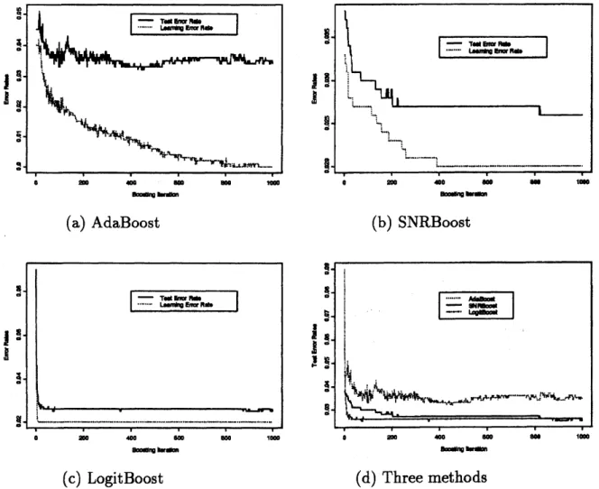
Figure 4: Comparison of three boosting methods in 2% mislabeled data far from
decision boundary, (a) Learning and test errorrates of AdaBoost. (b) Learning and
test error rates of SNRBoost. (c) Learning and test error rates of LogitBoost. (d)
Test error rates of three boosting methods.
We plot in Figures 4 the learning (error minimization) curves for 2% mislabeled
data in far case, and in Figures 5 that for 2% mislabeled data in near case. In each
figure, (a) shows AdaBoost learning and test error rates, (b) learning and test error
rates of the proposed method, (c) learning and test error rates of the LogitBoost,
and (d) comparison of test error rates of allthe three boosting methods.
In Figures $4(\mathrm{a})$, AdaBoost learning error rate levels off into 0% around at 940
118
$i^{\mathrm{I}}\iota$ $=$..-
$\ldots$. $\mathrm{R}$ ${ }$ ....-
$\ldots$. $\tau$ $\mapsto$ ! . $.\underline{}$ ‘ $*$$.-$
..
.: ..-$\cdot$$\cdot\cdot--\cdots\ldots\ldots..-\cdot\cdot\cdotrightarrow-\cdots\ldots-\cdot$ 0 0 ’ 0(a) AdaBoost (b) SNRBoost
$_{}.$
..
$\cdots.\ldots----\mathrm{T}$ $\ldots\ldots..---\cdot-\cdot-$ \S $|\downarrow.\eta||1|$ $\vdash|$ \S $|_{1\mathrm{l}}1_{1^{1}}’\downarrow \mathrm{r}_{d}$$\backslash \cdot...-\dot{j^{-}‘}..-\cdot.-\sim t_{-}-,\cdot\cdot-\cdots\underline{\dot{}\underline{i_{\dot{}}}}-_{\dot{\mathrm{H}}}$
${ }$ . $’\ldots\neg l$ -
...
$-\cdot..\dot{_{}.}\mathrm{i}$ \S 0n$\cdot \mathrm{w}\mathrm{u}\mathrm{m}\ovalbox{\tt\small REJECT}$
o ’
laanhg$\cdot\infty \mathrm{I}$
’
(c) LogitBoost (d) Three methods
Figure5: Comparison of three boostingmethodsin2% mislabeleddataneardecision
boundary, (a) Learningand test errorrates ofAdaBoost. (b) Learning and testerror
rates of SNRBoost. (c) Learning and test error rates of LogitBoost. (d) Test error
Figure $4(\mathrm{b})$, SNRBoost learning error rate falls into 0.02% and test error rate into
0.026%. In Figure$4(\mathrm{c})$, LogitBoost learningerror rate falls into 0.02% and testerror
rate into 0.025%. These facts dipict that SNRBoost and LogitBoost both succeeded
inlowering test error rate. InFigure$4(\mathrm{d})$, thetest errorrateofSNRBoost issuperior
to AdaBoost and it exhibits equal performance to LogitBoost.
In Figures 5, the peformance of three boosting method for 2% mislabeled data
in near case is shown. In Figure $5(\mathrm{a})$, AdaBoost learning error rate levels off into
0% around at 400 round and test error rate is fluctuating around 0.03%. In Figure
$5(\mathrm{b})$, SNRBoost learning error rate falls into 0.017% at 1000 round and test error
rate into 0.025%. In Figure $5(\mathrm{c})$, LogitBoost learning error rate falls into 0.01%
and test error rate into 0.03%. From learning error rates of all the three boosting
methods, we may observe that the mislabeled data near the dicision boundary is
easier to classify than the mislabeled datafar fromthe decision boundary. In Figure
$5(\mathrm{d})$, test error rate of SNRBoost is superior to the other two boosting methods.
The performance of LogitBoost is not as good as that in the far case. This may
be due to the fact that the mislabeled data near the dicision boundary is easier to
classify. In summary, SNRBoost exhibits a higher capability for generalization.
5.
Conclusion
We developed a new, robust boosting method against mislabeled, noisy data. The
newformulation uses the misclassification loss function, i.e., zer0-0ne loss function.
In deriving the algorithm, Stochastic Noise Reaction technique (Koda and Okano,
2000) is used to approximate the derivative of the zer0-0ne loss function.
Perfor-mance of theproposed method is compared with that of AdaBoost and LogitBoost
throughintensive numerical experiments. The proposed method is robust compared
to the other two boosting methods especialy in the mislabeled data near dicision
boundary. Even for mislabed datafar from decision boundary, the proposed method
exhibits the similar performance with that of LogitBoost.
Acknowledges
We thank Hiroyuki Okano for useful comments on an earlier draft. The work of M.
Koda and H.Suzuki is supported in part by a Grant-in-Aid for Scientific Research
of the Ministry ofEducation, Culture, Sports, Science and Technology of Japan.
References
Breiman, L. (1998): Combining Predictors. Technical Report, Statistics
Depart-ment, University of California, Berkeley.
$\mathrm{D}\mathrm{a}\mathrm{c}\mathrm{o}\mathrm{l},\mathrm{D}.\mathrm{K}$
.
andRabitz, H. (1984): Sensitivityanalysisofstochastic kineticmodels.120
Duda, R.O and Hart, P. E. and $\mathrm{S}\mathrm{t}\mathrm{o}\mathrm{r}\mathrm{k},\mathrm{D}$
.
G.(2001): Pattern Classification, JohnWiley
&
Sons, New York, $\mathrm{N}\mathrm{Y}$.
Fournie, E. Lasry, $\mathrm{J}.\mathrm{M}$, Lebuchoux $\mathrm{J}$, Lions, $\mathrm{P}.\mathrm{L}$, Touzi, N. (2001): Applications of
Malliavin calculus to monte carlo methods in finance. FinanceStochast., 5, 201-236.
Freund, Y. (1995): Boosting a weak learning algorithm by majority.
Information
and Computation, 121 (2),
256-285.
Freund, Y. and Schapire, R. E. (1997): Adecision-theoreticgeneralization of online
learning andanapplication to boosting. Journal
of
Computerand SystemSciences,55 (1), 119-139.
Friedman, J. (2001): Greedy function approximation: A gradient boosting
ma-chine. Annals
of
Statistics, 29 (5), 1189-1232.Friedman, J., Hastie, T., and Tibshirani, R. (2000): Additive logistic regression: a
statistical view ofboosting. Annals
of
Statistics, 28 (2), 337-407.Grove, A. and Schuurmans, D. (1998): Boosting in the limit: Maximizing the
mar-gin oflearned ensembles. Proc. 15th National
Conference
onArtifical
Intelligence,692-699.
Hastie, T., Tibshirani, R. and Friedman, J. (2001): The Elements of Statistical
Learning: Data Mining, Inference and Prediction. Springer, New York, $\mathrm{N}\mathrm{Y}$
.
Koda, M. and Okano, H. (2000): A new stochastic learning algorithm for neural
networks. Journal
of
the Operations Research Societyof
Japan, 43 (4), 469-485.Mason, L., Bartlett, P. L., and Baxter, J. (2000): Improved generalization through
explicit optimization of margins. Machine Learning, 38 (3), 243-255.
Mason, L., Baxter, J., Bartlett, P. L., and Frean, M. (2000): Functional gradient
techniques for combining hypotheses. In A.J.Smola, P.L.Bartlet, B.Scholk\"opt, and
D. Schuurmans, editors, Advances in Large Margin Classifiers, pages 221-246. MIT
Press, Cambridge, MA, 2000.
Novikov $\mathrm{E}\mathrm{A}$
.
(1965): Functional$\mathrm{s}$ and the random-force method in turbulence
theoty. $Sov$ Phys JETP, 20, 1290-1294.
Okano, H. and Koda, M. (2003): An optimization algorithm based on
stochas-tic sensitivity analysis for noisy objective landscapes. Reliability Engineering and
System Safety, 79 (2), 245-252.
Quinlan, J. R. (1996): Boosting first-0rder learning. Proc. 7th International
R\"atsch, G., Onoda, T., and Muller, K.-R. (2001): Soft margin for AdaBoost.
Machine Learning, 42 (3), 287-320.
Schapire, R. E. (1990): Thestrength ofweaklearnability. Machine Learning, 5 (2),