The
matrix coefficients
of the large discrete
series
of
$SU$(3,1)
早田 孝博(山形大) Takahiro HAYATA (Yamagata Univ.)
古関 春隆(三重大) Harutaka KOSEKI (Mie Univ.)
織田 孝幸 (東京大)1 Takayuki ODA (Univ. of Tokyo)
1. INTRODUCTION
This is an announcement of the forthcoming paper [HKO3]. In this paper we present
the explicit formula of matrix coefficients of the large discrete series representations of
$SU(3,1)$, the unitary group of signature $(3+, 1-)$ without proofs.
In the theory of automorphic forms, the dimension formula is of a great concern. In
the situation of hermitian symmetric domains of type I, there is a result of Suehiro
Kato [Kl, K2] when the group is the special unitary group of signature $(p+, 1-)$ which
treats a dimension formula of holomorphic automorphic forms. This form stems from
so-called (anti-)holomorphic discrete series representations of this $\mathbb{Q}$-rank 1 semi-simple
Lie group. With representation theoretical view, there is a non-holomorphic discrete
series, or “large“ discrete series representation. The Selberg-Godement’s formula [Go],
which computes the dimension of bounded automorphic forms, requires no assumption
for discrete series except integrability. However, the computationof kernel functionat the
“large” case seems still open. This is because we think the combinatorics of the weight
basis of $U(3)$ would remain hard. On the other hand, in the papers $[HiO, HiO2]$ there is
a nice way to treat these basis in very concrete fashion. By using this, we calculate the
matrix coefficients of$SU(3,1)$ in this paper.
The content of this paper is as follows. In Section 2 we treat the matrix coefficients
of the discrete series in general. Then the Dirac-Schmid equations are introduced. In
Section 3, we introduce the unitary group $SU(3,1)$ and its Lie algebra. Then the discrete
series of $SU(3,1)$ is introduced concretely. We need the Harish-Chandra parameter, the
Blattner parameter and the associated non-compact roots.
In Section 4, the canonical basis of$GL(3)$ is introduced. It is described using
Gel‘fand-Tsetlin pattern, and also called Gel‘fand-Zelevinsky basis. Since the matrix coefficients
reflect detailed geometric nature ofweight basis, we investigate the weight diagram very
closely.
In Section 5, we specify the Dirac-Schmid equality by the $SU(3,1)$-data. We compute
the injectors in avery concrete way. In Section 6 the main results of this paper are given.
We select the $\mathbb{Q}$-generating set of matrix coefficients, which we call standard
functions
(Theorem 6.3). Then the problem to compute matrix coefficients is reduced to that of
standardfunctions. Thestandard functionsaredescribed bythehypergeometric functions
$2F1$ (Proposition 6.8 and Lemma 6.12). We state these main results without proofs. The
detailed ingredients are discussed in forthcoming paper [HKO3].
Notation. $\mathbb{Z},$ $\mathbb{Q},$ $\mathbb{R}$ and $\mathbb{C}$ are the ring of integers, the fields of rational numbers, real
numbers and complex numbers. Let $M_{n}(\mathbb{C})$ be the space of complex square matrices of
degree$n$. Then $E_{ij}$ denotes the matrix units with 1 at the $(i,j)-$th entry and
zeros
at theother entries.
2. GENERALITIES
2.1. Spherical functions or matrix coefficients belonging to the discrete series.
Let $G$ be a real semi-simple Lie group of finite center. Let $K$ be a maximal compact
subgroup of $G$. We
assume
that $G$ has a compact Cartan subgroup $T$. Let $L^{2}(G)$ be the$L^{2}$-space ofmeasurable functions on $G$ with respect to the Haar-Hurwitz measure, which
is a $G\cross G$ bi-module with the action
$\mathcal{L}(g_{1})\mathcal{R}(g_{2})\varphi(x):=\varphi(g_{1}^{-1}xg_{2})$ $(\varphi\in L^{2}(G), x\in G, (g_{1}, g_{2})\in G\cross G)$
.
The discrete series representations are, by definition, in the sum of the closed invariant
subspace under this action of $G\cross G$. With this definition and from the results of
Harish-Chandra, we have the discrete series
$L^{2}(G)_{d}:= \bigoplus_{-\lambda\in_{-}^{-}}\pi_{\lambda}^{*}\otimes\pi_{\lambda}$
as $G\cross G$ bi-module, with parameters $\lambda$ in the dominant regular integral weights $\Xi$ with
respect to a compact Cartan subalgebra $t=$ Lie$T$ (Harish-Chandra parameters).
Let $(\pi_{\lambda}, H_{\lambda})$ be a discrete series representation with Harish-Chandraparameter
$\lambda$. Let $\mathcal{T}:\pi_{\lambda}^{*}$
rz
$\pi_{\lambda}arrow L^{2}(G)$ be the unique$G\cross G$ homomorphism up toconstant multiple. If wedenote by
$\langle$ , $\}:H_{\lambda}^{*}\cross H_{\lambda}arrow \mathbb{C}$
be the G-equivariant canonical coupling, then $\mathcal{T}$ is given as
$\mathcal{T}(v^{*}\otimes v)(x)=\{v^{*}, \pi(x)v\}$ for $v\in H_{\lambda}$ and $v^{*}\in H_{\lambda}^{*}$,
because we can check the intertwining property
$\mathcal{L}(g_{1})\mathcal{R}(g_{2})\mathcal{T}(v^{*}\otimes v)(x)=\mathcal{T}((\pi_{\lambda}^{*}(g_{1})v^{*}$図 $\pi_{\lambda}(g_{2})v)(x)$
immediately.
Let $\iota:W_{\tau}arrow H_{\lambda}$ and $\iota^{*}:W_{\tau^{*}}arrow H_{\lambda}^{*}$ be $K$ modules and K-injections. Then we define
the matrix
coefficients of
$\pi_{\lambda}$ with K-type $\tau$ at vector $f\otimes f’$ by$c(f\otimes f’;x):=\mathcal{T}(\iota^{*}(f’)\otimes\iota(f))(x)$
Since $G$ has a Cartan decomposition $G=KAK$, where $A$ is the connected component
of split R-torus of $G$, the matrix coefficients $c(f\otimes f’;x)$ can be determined by the value
at $a_{r}\in A$, which we call the radial component.
2.2. The Dirac-Schmid equations. Let $\tau$ be a multiplicity-one K-type of $\pi_{\lambda}$ and
let $\tau^{(e)}$ be a constituent of Ad$(K)\otimes\tau$ and $I^{(e)}:\tau^{(e)}arrow \mathfrak{p}_{\mathbb{C}}\otimes W_{\tau}$ be an injective
K-homomorphism. If $\tau^{(e)}$ is not a constituent of $\pi_{\lambda}|K$ then for each $I^{(e)}(f)= \sum_{i}X_{i}\otimes v_{i}$,
we have
$\sum_{i}\mathcal{R}_{X_{i}}\mathcal{T}(\iota^{*}(v^{*})\otimes\iota(v_{i}))=0$
$(v^{*}\in H_{\pi_{\lambda}}^{*})$
since $\tau^{(e)}arrow \mathfrak{p}_{\mathbb{C}}\otimes W_{\tau}arrow H_{\pi}$ becomes also a K-homomorphism. We call this the (right)
3. THE UNITARY GROUP $SU(3,1)$, ROOT SYSTEMS AND THE HARISH-CHANDRA PARAMETERS
3.1. The Lie group and the Lie algebra. The Lie group $G:=SU(3,1)$ is realized as
$\{g\in M_{4}(\mathbb{C})|{}^{t}\overline{g}1_{3,1}g=1_{3,1}, \det g=1\}$
with $1_{3,1}=$ diag$(1, 1, 1,$ $-1)$, and its Lie algebra $\mathfrak{g}:=\mathfrak{g}u(3,1)$
.
We choose a Cartan involution
$\theta:g\in G\mapsto\iota_{\overline{g}^{-1}}\in G$,
and the induced involution on the Lie algebra:
$\theta:X\in \mathfrak{g}\mapsto-{}^{t}X^{-}\in g$
.
Fix a compact Cartan subgroup $T$ in $K=G^{\theta}$ consisting of the diagonal matrices in $G$,
and let $g=oplus \mathfrak{p}$ be the Cartan symmetric decomposition. The adjoint action ofa central
elementsdiag$(z, z, z, z^{-3})$ with $z=\exp(\pi\sqrt{-1}/8)$ defines the canonical complex structure
on $\mathfrak{p}$. Then the $(+1, -1)$ part $\mathfrak{p}_{+}$ and the $(-1, +1)$ part p-in $\mathfrak{p}\otimes \mathbb{C}$ is given by
$\mathfrak{p}_{+}=\mathbb{C}E_{14}\oplus \mathbb{C}E_{24}\oplus \mathbb{C}E_{34}$, $\mathfrak{p}_{-}=\mathbb{C}E_{41}\oplus \mathbb{C}E_{42}\oplus \mathbb{C}E_{43}$.
Let $a$ be a maximal abelian subalgebra in $\mathfrak{p}$ generated by $H_{a}=E_{14}+E_{41}$. We set
$A=\exp(a)$.
We put $M$ $:=Z_{K}(A)$ the centralizer of$A$ in $K$:
$M=\{(u_{1} U_{2} u_{4})|u_{1}\in U(1),$ $U_{2}\in U(2),$ $u_{4}=u_{1},$ $u_{1}^{2}\det(U_{2})=1\}$ ,
which is isomorphic to $U(1)\cross U(2)$.
3.2. The $ro$ot systems. The unitary characters of the compact Cartan subgroup
$T$ $:=\{t$ $:=$ diag$(u_{1},$$u_{2},$ $u_{3},$ $u_{4})|u_{i}\in U(1),$ $u_{4}=(u_{1}u_{2}u_{3})^{-1}\}$
are expressed as
$\chi:T\ni t\mapsto\prod_{i=1}^{3}u_{i}^{l_{i}}\in U(1)$,
with some triple ofintegers $(l_{1}, l_{2}, l_{3})\in Z^{3}$
.
The root system $\Phi(g_{\mathbb{C}},$$\{c)$ is given by $\{\beta_{ij}(i\neq j)\}$ with $\beta_{ij}(t)=u_{i}/u_{j}(1\leq i,j\leq 3)$
which is of type $A_{3}$.
$\mathbb{R}om$ now on we fix as a positive system $\Phi^{+}:=\{\beta_{ij}(i<j)\}$. Then two compact roots
$\beta_{12}=(1, -1,0)$ and $\beta_{23}=(0,1, -1)$ and a non-compact root $\beta_{34}=(1,1,2)$ form the
simple roots in this positive system. Note that $\rho$ the half sum of positive roots is given
by $\rho=(3,2,1)$
.
3.3. Harish-Chandraparametrization. We recall here the
Harish-Chandra
parametriza-tion of the discrete series representations for $SU(3,1)$ and their minimal K-types.
The set of finite-dimensional irreducible representations of $K$ is parametrized by a
subset $\Xi$ of integral weights $L_{T}=Hom(T, U(1))$ of the representations of $K$, which
are
dominant, i.e., its parameter is ofthe form $(l_{1}, l_{2}, l_{3})\in Z^{3}$ satis$\mathfrak{h}ringl_{1}\geq l_{2}\geq l_{3}$
.
Since $T$ is also a Cartan subgroup of $G$, the Killing form on $\mathfrak{g}$ restricted to
$t$ defines
the natural inner product on $L_{T}$:
$(l, l’):= \sum_{i=1}^{3}l_{i}l_{i}’-\frac{1}{4}(\sum_{i=1}^{3}l_{i})(\sum_{i=1}^{3}l_{i}’)$
.
The set ofequivalence classes of the discrete series representations of$G$is parametrized
byasubset of$L_{T}+\rho=L_{T}$, whichis positivewithrespect compact positiveroots$\{\beta_{12}, \beta_{23}\}$
.
There are 4 different positive systems in $\Phi(g, t)$ compatible with the positive system of
compact roots generated by simple roots $\{\beta_{12}, \beta_{23}\}$; these are specified by 4 simple root
systems $\Delta_{J}(J\in\{I, II, III, IV\})$:
(I) $:\{\beta_{12}, \beta_{23},\beta_{34}\}$; (II) $:\{\beta_{12}, \beta_{24}, \beta_{43}\}$;
(III) : $\{\beta_{14}, \beta_{42}, \beta_{23}\}$; (IV) : $\{\beta_{41}, \beta_{12}, \beta_{23}\}$
with the corresponding sets of positive non-compact roots $\Phi_{J,n}$:
(I) : $\Phi_{I,n}^{+}=\{\beta_{14}, \beta_{24}, \beta_{34}\}$; (II) : $\Phi_{II,n}^{+}=\{\beta_{14}, \beta_{24}, \beta_{43}\}$;
(III) : $\Phi_{III,n}^{+}=\{\beta_{14}, \beta_{42}, \beta_{43}\}$; (IV) : $\Phi_{lV,n}^{+}=\{\beta_{41}, \beta_{42}, \beta_{43}\}$
.
And the halfsum of positive roots $\rho_{J}$ for each $J$ is given by
$\rho_{I}=\rho=(3,2,1)$; $\rho_{II}=(2,1, -1)$; $\rho_{III}=(1, -1, -2)$; $\rho_{IV}=(-1, -2, -3)$
.
Here we set
$\Xi=\Xi_{I}\cup\Xi_{II}\cup\Xi_{III}\cup\Xi_{IV}$.
with
三I $:=\{l=(l_{1}, l_{2}, l_{3})\in L_{T}|l_{1}>l_{2}>l_{3}>0\}$, $\Xi_{II}:=\{l\in L_{T}|l_{1}>l_{2}>0>l_{3}\}$, $\Xi_{III}:=\{l\in L_{T}|l_{1}>0>l_{2}>l_{3}\}$, $\Xi_{IV}:=\{l\in L_{T}|0>l_{1}>l_{2}>l_{3}\}$
.
For each element $\lambda\in\Xi_{J}$, there is the unique discrete series representation $\pi_{\lambda}$, which
is specified by its character formula of $T$. The minimal K-type $\mu$ of $\pi_{\lambda}$ is given by
$\mu=\lambda+\rho_{n}(\lambda)-\rho_{c}=\lambda+\rho(\lambda)-2\rho_{c}$. Note here that $2\rho_{c}=(2,0, -2)$, i.e., $\rho_{c}=(1,0, -1)$.
4. THE $GEL’ FAND$-ZELEVINSKY BASIS FOR SIMPLE $GL(3)$-MODULES
Recall the paper [GZ] of Gel‘fand-Zelevinsky and the previous papers $[HiO, HiO2]$.
Given a highest weight $\mu$, we get a highest weight module $(\tau_{\mu}, W_{\mu})$ of$GL(3)$. Let $W(\mu)$
be the set of weights in $(\tau_{\mu}, W_{\mu})$
.
For its weight basis, we can associate the set $G(\mu)$ ofthe Gel‘fand-Tsetlin patterns $M$:
Thenaccording to [GZ],thesimpleK-module $V_{\mu}$ofhighest weight$\mu$hasabasis$\{f_{\mu}(M)|M\in$
$G(\mu)\}$, which is called a Gel‘fand-Zelevinsky basis.
Fromnowon,weusetheoffsetnotationforGel ifand-Tsetlin patterns (i.e., GT-patterns):
$M(\begin{array}{l}a,bc\end{array})=(\begin{array}{lll}\mu_{l} \mu_{2_{\prime}} \mu_{3}m_{l2}+a m_{22}+b m_{1l}+c \end{array})$ for $M=(\begin{array}{ll}\mu_{2}\mu_{1}, \mu_{3}m_{12} m_{22}m_{11} \end{array})$ and the offset $(\begin{array}{l}a,bc\end{array})$ .
Moreover the symbol $M[a]$ means $M(\begin{array}{ll}a -a 0\end{array})$. We also denote $\mu_{i}=m_{i3}(i=1,2,3)$
.
The weight $wt(M)$ of the GT-pattern $M$ is given as
$(m_{11}, m_{12}+m_{22}-m_{11}, \sum_{i=1}^{3}\mu_{i}-(m_{12}+m_{22}))$
Note that $wt(M[a])=wt(M)$. We sometimes identify the basis $f_{\mu}(M)$ with the
GT-pattern $M$ when the highest weight $\mu$ is clear from the context.
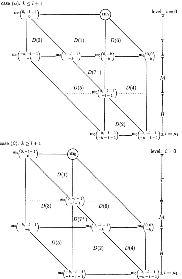
4.1. Decomposition of the weight polygon. Given a dominant integral weight $\mu=$
$(\mu_{1}, \mu_{2}, \mu_{3})\in Z^{3}(\mu_{1}\geq l^{\iota_{2}}\geq\mu_{3})$, the convex closure ofall the permutations $(\mu_{a}, \mu_{b}, \mu_{c})$ of
three components of $\mu$ $(\{a, b, c\}=\{1_{\}}2,3 \})$ generically makes a hexagon Hex$(\mu)$ in the
plane $\{(x_{1}, x_{2}, x_{3})\in R^{3}|\sum_{i}x_{i}=\sum_{i}\mu_{i}\}$ ofthe Euclidean 3-space. If$\mu_{1}=\mu_{2}=\mu_{3}$, this
is a point, and when either $\mu_{1}>\mu_{2}=\mu_{3}$ or $\mu_{1}=\mu_{2}>\mu_{3}$ it is a triangle.
Then the intersection Hex$(\mu)\cap Z^{3}$ coincides with the set ofweights $W(\mu)$ belonging to
the highest weight $\mu$. We divide this set into seven parts in the following manner.
$D(1):=\{w=(w_{1},$$w_{2},$ $w_{3})\in W(\mu)|w_{1}\geq\mu_{2},$ $w_{2}\leq\mu_{2}$, and $w_{3}\leq\mu_{2}\}$,
$D(3):=\{w=(w_{1},$$w_{2},$$w_{3})\in W(\mu)|w_{1}\geq\mu_{2},$ $w_{2}\leq\mu_{2}$, and $w_{3}\geq\mu_{2}\}$,
$D(6):=\{w=(w_{1},$$w_{2},$$w_{3})\in W(\mu)|w_{1}\geq\mu_{2},$ $w_{2}\geq\mu_{2}$, and $w_{3}\leq\mu_{2}\}$,
$D(4):=\{w=(w_{1},$ $w_{2},$$w_{3})\in W(\mu)|w_{1}\leq\mu_{2},$ $w_{2}\geq\mu_{2}$, and $w_{3}\leq\mu_{2}\}$,
$D(5):=\{w=(w_{1},$$w_{2},$$w_{3})\in W(\mu)|w_{1}\leq\mu_{2},$ $w_{2}\leq\mu_{2}$, and $w_{3}\geq\mu_{2}\}$,
$D(2):=\{w=(w_{1},$$w_{2},$$w_{3})\in W(\mu)|w_{1}\leq\mu_{2},$ $w_{2}\geq\mu_{2}$, and $w_{3}\geq\mu_{2}\}$,
$D(7^{+})$ $:=\{w=(w_{1},$$w_{2},$$w_{3})\in W(\mu)|w_{i}\geq\mu_{2}$, for all $i\}$,
$D(7^{-}):=\{w=(w_{1},$$w_{2},$$w_{3})\in W(\mu)|w_{i}\leq\mu_{2}$, for all $i\}$.
Let $w=(w_{1}, w_{2}, w_{3})$ be a weight belonging to a highest weight $\mu$. Then the set of
GT-patterns belonging to $w$ is of the form
$G(\mu;w):=\{M[-t]|t\in \mathbb{Z}\cap[a, b]\}$
with some G-pattem $M$ and
some
integers $a,$ $b$. In particular, we may choose $M$ and$a$ such that $a=0$
.
Then $M$ is called the leading GT-pattem belonging to the weight$w$. Moreover we call the difference $b-a$ the meson number $m(w)\geq 0$
of
the weight $w$.
Thereforethe cardinality of$G(\mu;w)$ is $m(w)+1$. We have $m(w) \leq\inf\{\mu_{1}-\mu_{2}, \mu_{2}-\mu_{3}\})$
and the equality $m(w)= \inf\{\mu_{1}-\mu_{2},\mu_{2}-l^{l_{3}}\}$ is valid if and only if $w\in D(7^{+})$ or
Let $w=(w_{1}, w_{2}, w_{3})\in W(\mu)$ be
a
weight belonging to $\mu$.
Thenwe
call $i$ $:=\mu_{1}-w_{1}$the level of the weight $w$
.
Let $L(i)$ be the set ofweights of level $i$ in $W(\mu)$.
Then this isaline segment of at most length $k+l+1$.
We spell out explicitly all the weights belonging to each domain $D(J)(J=1, \cdots, 7)$.
The result is different depending on the
cases:
the
case
$(\alpha)$: $\mu_{1}-\mu_{2}=k\leq\mu_{2}-\mu_{3}=l+1$;the case $(\beta)$: $\mu_{1}-\mu_{2}=k\geq\mu_{2}-\mu_{3}=l+1$
.
In the former case wedenote $\mu=(k+l+1, l+1,0)\in(\alpha)$, and in thesecond case $\mu\in(\beta)$
.
If the first component $w_{1}=k+l+1-i$ ofthe weight $w\in W(\mu)$ belongs to the range
such that $0 \leq i\leq\inf\{k, l+1\}$,
we
say that the weight belongs to the top range, anddenote this by $w\in \mathcal{T}$symbolically; if$i$ satisfies $\inf\{k, l+1\}\leq i\leq\sup\{k, l+1\}$, then the
weight belongs to the middle range $(w\in \mathcal{M})$; lastly if$\sup\{k, l+1\}\leq i$, we say that the
weight belongs to the bottom range $(w\in \mathcal{B})$.
4.2. Parametrization of the Ieading GT-patterns. We write the exhaustive list of
theleading GT-patterns oneach $D(J)(1\leq J\leq 7)$. In what follows,wedefine the highest
weight vector $m_{0}:=(\begin{array}{ll}\mu_{l},\mu_{2} \mu_{3}\mu_{1} \mu_{2}\mu_{l} \end{array})$
.
We also set $c(i)=|l+1-i|$.
On $D(6)$:
(1) If $\mu\in(\alpha)$, or $\mu\in(\beta)$ and $w\in \mathcal{T}$, the leading GT-patterns in $D(6)$ is exhausted by
$M_{(a)}$ $:=m_{0}(\begin{array}{ll}0,-i+ a-i \end{array})$ $(0 \leq a\leq i\leq\inf\{k, l+1\})$
with $wt(M_{(a)})=(k+l+1-i, l+1+a, i-a),$ $\delta(M_{(a)})=a$, and the meson number
$m(M_{(a)})=i-a$
.
(2) The
case
$\mu\in(\beta)$ and $w\in \mathcal{M}$:$M_{(b)}:=m_{0}(\begin{array}{l}0,-l-l+b-i\end{array})$ $(l+1\leq i\leq k, 0\leq b\leq l+1)$
with$wt(M_{(b)})=(k+l+1-i, b+i, l+1-b),$ $\delta(M_{(b)})=-l-1+i+b$, and$m(M_{(b)})=l+1-a$.
On $D(3)$:
(1) If $\mu\in(\alpha)$, or if$\mu\in(\beta)$ and $w\in\tau$:
$M_{(a)}:=\mathfrak{m}(\begin{array}{ll}-a -l-1 -i\end{array})$ $(0\leq a\leq i\leq k)$
with $wt(M_{(a)})=(k+l+1-i, i-a, l+1+a),$ $\delta(M_{(a)})=-l-1+i-a$ and $m(M_{(a)})=i-a$.
(2) if $\mu\in(\beta)$ and $w\in \mathcal{M}$:
$M_{(b)}$ $:=m_{0}(\begin{array}{lll}l+l-i- b -l-1-i \end{array})$ $(l+1\leq i\leq k, 0\leq b\leq l+1)$
with $wt(M_{(b)})=(k+l+1-i, l+1-b,i+b),$ $\delta(M_{(b)})=-b$, and $m(M_{(b)})=l+1-b$.
On $D(4)$:
(1) If$\mu\in(\alpha)$ and $w\in \mathcal{M}$ :
case $(\alpha):k\leq l+1$
case $(\beta):k\geq l+1$
with $wt(M_{(a)})=(k+l+1-i, l+1+a,i-a),$ $\delta(M_{(a)})=a,$ $m(M_{(a)})=k-a$.
(2) If$\mu\in(\alpha)$ and $w\in \mathcal{B}$, or if$\mu\in(\beta)$:
$M_{(b)}:=m_{0}(\begin{array}{l}0,-l-l+b-i\end{array})$ $(k\leq i\leq k+l+1,0\leq b\leq k+l+1-i)$
with $wt(M_{(b)})=(k+l+1-i, b+i, l+1-b),$ $\delta(M_{(b)})=-l-1+i+b$, and $m(M_{(b)})=$
$k+l+1-i-b$
. On $D(5)$:(1) $(\alpha)$ and $w\in \mathcal{M}$:
$M_{(a)}:=m_{0}(\begin{array}{ll}-a -l-l -i\end{array})$ $(0\leq a\leq k\leq i\leq l+1)$
with $wt(M_{(a)})=(k+l+1-i, i-a, l+1+a)$ and$\delta(M_{(a)})=-l-1+i-a,$ $m(M_{(a)})=k-a$.
(2) If $(\alpha)$ and $w\in \mathcal{B}$, or if$\mu\in(\beta)$:
$M_{(b)}:=m_{0}(\begin{array}{ll}l+1-i-b -l-1-i \end{array})$ $(0\leq i-(l+1)\leq k, 0\leq b\leq k+l+1-i)$
with $wt(M_{(b)})=(k+l+1-i, l+1-b, i+b),$ $\delta(M_{(b)})=-b$, and $m(M_{(b)})=k+l+1-i-b$
.
On $D(1)$, the forms of theleading GT-patterns arethe sameinthe both
cases
$(\alpha),$ $(\beta)$.But the range of the parameters are different.
$M_{[a]}:=m_{0}(\begin{array}{ll}0,-i- a-i \end{array})$ $(0\leq i\leq id\{k, l+1\}, 0\leq a\leq l+1-i)$
with $wt(M_{[a]})=(k+l+1-i, l+1-a,i+a),$ $\delta(M_{[a]})=-a,$ $m(M_{[a]})=i$.
On $D(2)$ we have the same form of GT-patterns with different ranges of parameter
depending on the $(\alpha)$ case or $(\beta)$
case.
$M^{[b]}:=m_{0}(\begin{array}{ll}-i+(l+1)+b -l-1-i \end{array})$ $( \sup\{k, l+1\}\leq i\leq k+l+1,0\leq b\leq i-(l+1))$
with $wt(M^{[b]})=(k+l+1-i, l+1+b, i-b),$ $\delta(M^{[b]})=b,$ $m(M^{[b]})=k+l+1-i$
.
On $D(7)$
we
have the following selections:$(\alpha)$ : $M_{[a]}=m_{0}(\begin{array}{ll}0,-i- a-i \end{array})$ $(k\leq i\leq l+1,0\leq a\leq l+1-i)$,
$(\beta)$ : $M^{[b]}=m_{0}(\begin{array}{ll}-i+(l+1)+b -l-l-i \end{array})$ $(l+1\leq i\leq k, 0\leq b\leq i-(l+1))$.
The weights and $\delta$ are given in the formulas in the domains $D(1)$ and $D(2)$. Moreover
the meson number is $\inf\{k, l+1\}$.
5. DIRAC-SCHMID EQUATIONS ON $SU(3,1)$
Let $(\tau_{\mu}, W_{\mu})$ be the minimal K-type of $(\pi_{\lambda}, H_{\lambda})$. The action of the basis $E_{ij}(i,j=$
Proposition 5.1 (Gel‘fand-Zelevinsky). Let $f_{\mu}(M)$ be the basis with GT-pattern $M\in$
$G(\mu)$. The action
of
the six weight vectors $E_{ij}(i\neq j)$ is given asfollows; $E_{12}f_{\mu}(M)=(m_{12}-m_{11})f_{\mu}(M(^{0}i^{0}))+(m_{23}-m_{22})\chi_{+}(M)f_{\mu}(M(\begin{array}{l}0,0l\end{array})[-1])$ , $E_{21}f_{\mu}(M)=(m_{11}-m_{22})f_{\mu}(M(\begin{array}{l}0,0-l\end{array}))+(m_{12}-m_{23})\chi_{-}(M)f_{\mu}(M(\begin{array}{l}0,0-1\end{array})[-1])$, $E_{23}f_{\mu}(M)=(m_{13}-m_{12})f_{\mu}(M(\begin{array}{l}l,00\end{array}))+(m_{13}-m_{12}-\delta(M))\chi_{-}(M)f_{\mu}(M(\begin{array}{l}l,00\end{array})[-1])$, $E_{32}f_{\mu}(M)=(m_{22}-m_{33})f_{\mu}(M(0 -l0))+(m_{22}-m_{33}+\delta(M))\chi_{+}(M)f_{\mu}(M(\begin{array}{l}0,-l0\end{array})[-1])$ , $E_{13}f_{\mu}(M)=(m_{13}-m_{12})f_{\mu}(M(\begin{array}{l}l,0l\end{array}))-\overline{c}_{1}(M)f_{\mu}(M(\begin{array}{l}1,0l\end{array})[-1])$, $E_{31}f_{\mu}(M)=-(m_{22}-m_{33})f_{\mu}(M(\begin{array}{l}0,-l-l\end{array}))+c_{1}(M)f_{\mu}(M(\begin{array}{ll}0 -l-l \end{array})[-1])$ . Here we set $\delta(M):=m_{12}+m_{22}-m_{11}-m_{23}$, and$\chi_{+}(M)=\{\begin{array}{ll}1, if \delta(M)>00, otherwe\end{array}$ ;
Moreover
$\chi_{-}(M)=\{\begin{array}{ll}1, if \delta(M)<00, otherwise\end{array}$
$c_{1}(M)= \inf\{m_{11}-m_{22}, m_{12}-m_{23}\},\overline{c}_{1}(M)=\inf\{m_{23}-m_{22}, m_{12}-m_{11}\}$.
The actions
of
$E_{11},$$E_{22}$ and $E_{33}$ are given by$E_{11}f_{\mu}(M)=m_{11}f_{\mu}(M)$, $E_{22}f_{\mu}(M)=(m_{12}+m_{22}-m_{11})f_{\mu}(M)$,
$E_{33}f_{\mu}(M)=( \sum_{i=1}^{3}m_{i3}-m_{12}-m_{22})f_{\mu}(M)$.
For our later purpose, we introduce more piecewise linear functions:
$D(M)=m_{12}-m_{13}-\delta(M)$, $\overline{D}(M)=m_{33}-m_{22}+\delta(M)$, $c_{2}(M)=c_{1}(M)\overline{c}_{1}(M)$.
Proposition 5.2. Let $(\tau_{\mu}, V_{\mu})$ be the simple K-module with a dominant integral weight
$\mu=(m_{13}, m_{23}, m_{33})\in Z^{3}$, which is equippedwith an Gelfand-Zelevinsky basis$\{f_{\mu}(M)|M\in$ $G(\mu)\}$
.
Set $\mu^{(i)}=\mu+e_{i}$ and$\mu^{(-i)}=\mu-e_{i}(i=1,2,3)$, and let $\{f^{(\pm i)}(M)|M\in G(\mu^{(\pm i)})\}$be a Gel ‘fand-Zelevinsky basis
of
$V_{\mu^{(\pm i)}}$.(1) Up to a scalar multiple, the injector $V_{\mu+e_{3}^{c}}arrow V_{e_{1}}\otimes V_{\mu}$ is given by
$f_{\mu+e_{3}}(M’)=(\begin{array}{l}1,0l\end{array})\otimes f_{\mu}(m(\begin{array}{ll}0 -l-l \end{array}))-(\begin{array}{l}1,00\end{array})\otimes\{f_{\mu}(m(\begin{array}{l}0,-l0\end{array}))+\chi_{+}(M’)f_{\mu}(m(\begin{array}{l}-1,00\end{array}))\}$
$+(\begin{array}{l}0,00\end{array})\otimes f_{\mu}(m(\begin{array}{l}0,00\end{array}))$ .
(2) Up to a scalar multiple, the injector $V_{\mu+e_{2}}\mapsto V_{e_{1}}\otimes V_{\mu}$ is given by
$(d_{2}+1)f_{\mu+e2}(M’)=(\begin{array}{l}1,01\end{array})\otimes\{-(m_{22}’-m_{33}^{l})f_{\mu}(m(\begin{array}{l}0,-1-l\end{array}))+\chi_{-}(M’)\overline{D}(M’)f_{\mu}(m(\begin{array}{l}-1,0-1\end{array}))\}$
$+(\begin{array}{l}1,00\end{array})\otimes\{(m_{22}’-m_{33}’)f_{\mu}(m(\begin{array}{l}0,-l0\end{array}))-\overline{c}_{1}(M’)f_{\mu}(m(\begin{array}{l}-l,00\end{array}))\}$
$+(\begin{array}{l}0,00\end{array})\otimes\{(m_{23}’-m_{22}’)f_{\mu}(m(\begin{array}{l}0,00\end{array}))+\chi_{-}(M’)\overline{c}_{1}(M^{l})f_{\mu}(m(\begin{array}{l}-1,10\end{array}))\}$.
for
each $M’=(\mu+e_{2};m)\in G(\mu+e_{2})$. Here $\overline{D}(M’)=-(m_{22}’-m_{33}’)+\delta(M’)$.(3) The injector $V_{\mu+e_{1}}\mapsto V_{e_{1}}\otimes V_{\mu}$ is given by
$(d_{1}+1)(d_{1}+d_{2}+1)f_{\mu+e_{1}}(M’)$
$=(\begin{array}{l}l,01\end{array})\otimes\{-(m_{13}’-m_{12}’)(m_{22}’-m_{33}’)f_{\mu}(m(\begin{array}{l}-0,1-1\end{array}))+\overline{E}(M’)f_{\mu}(m(_{-i^{0}}^{-1}))\}$
$+(\begin{array}{l}l,00\end{array})\otimes\{(m_{13}’-m_{12}’)(m_{22}’-m_{33}^{l})f_{\mu}(m(\begin{array}{l}0,-l0\end{array}))-\overline{F}(M’)f_{\mu}(m(\begin{array}{l}-l,00\end{array}))$
$+c_{2}(M^{l})f_{\mu}(m(\begin{array}{l}-2,l0\end{array}))\}$
$+(\begin{array}{l}0,00\end{array})\otimes\{(m_{13}’-m_{12}’)(m_{13}’-m_{12}’+1)f_{\mu}(m)-c_{2}(M’)f_{\mu}(m(\begin{array}{l}-l,l0\end{array}))\}$
.
(4) The injector $V_{\mu-e_{1}}arrow V_{-e_{3}}\otimes V_{\mu}$ is given by
$f_{\mu-e_{1}}(M’)=(\begin{array}{l}0,00\end{array})\otimes f_{\mu}(M(\begin{array}{l}0,00\end{array}))-(o -l0)\otimes\{f_{\mu}(M(\begin{array}{l}l,00\end{array}))+\chi_{-}(M’)f_{\mu}(M(\begin{array}{l}0,l0\end{array}))\}$
$+(\begin{array}{l}0,-1-l\end{array})\otimes f_{\mu}(M(\begin{array}{l}1,0l\end{array}))$
.
(5) The injector $V_{\mu-e_{2}^{\zeta}}arrow V_{-e_{3}}\otimes V_{\mu}$ is given by
$(d_{1}+1)f_{\mu-e_{2}}(M’)=(\begin{array}{l}0,00\end{array})\otimes\{(m_{12}’-m_{23}^{l})f_{\mu}(M(\begin{array}{l}0,00\end{array}))+\chi_{+}’(M’)c_{1}(M’)f_{\mu}(M(\begin{array}{l}-1,l0\end{array}))\}$
$+(\begin{array}{l}0,-10\end{array})\otimes\{(m_{13}’-m_{12}’)f_{\mu}(M(\begin{array}{l}1,00\end{array}))-c_{1}(M’)f_{\mu}(M(\begin{array}{l}0,10\end{array}))\}$
$+(\begin{array}{l}0,-l-l\end{array})\otimes\{-(m_{13}’-m_{12}’)f_{\mu}(M(\begin{array}{l}l,0l\end{array}))+\chi_{+}’(M’)D(M’)f_{\mu}(M(\begin{array}{l}0,l1\end{array}))\}$
.
(6) The injector $V_{\mu-e_{3}}\mapsto V_{\mu-e_{3}}\otimes V_{\mu}$ is given by
$(d_{1}+1)(d_{1}+d_{2}+1)f_{\mu^{-e}3}(M’)$
$=(\begin{array}{l}0,00\end{array})\otimes\{(m_{12}’-m_{33}’+1)(m_{22}’-m_{33}’)f_{\mu}(M(\begin{array}{l}0,00\end{array}))-c_{2}(M’)f_{\mu}(M[-1])\}$
$-(0 l0)\otimes\{-(m_{13}’-m_{12}’)(m_{22}’-m_{33}’)f_{\mu}(M(\begin{array}{l}1,00\end{array}))+F(M’)f_{\mu}(M(\begin{array}{l}0,l0\end{array}))$
$-\chi_{-}(M’)c_{2}(M’)f_{\mu}(M(\begin{array}{l}l,00\end{array})[-2])\}$
$+(\begin{array}{ll}0 -l-1 \end{array})\otimes\{-(m_{13}’-m_{12}’)(m_{22}’-m_{33}’)f_{\mu}(M(\begin{array}{l}1,01\end{array}))+E(M’)f_{\mu}(M(\begin{array}{l}0,l1\end{array}))\}$
.
5.1. The annihilators of the minimal K-types. In what follows, werestrict ourselves
to the case when the discrete series is from $\Xi_{II}$
.
Let $\mu$ be the Blattner parameter of $\pi_{\lambda}\in\Xi_{II}$
.
Then by the Blattner formula (provedHere
we
$co$nsider the action of$\mathfrak{p}_{\mathbb{C}}=\mathfrak{p}_{+}\oplus \mathfrak{p}_{-}$ ontheK-finite elements intherepresenationspace of $\pi_{\lambda}$,
more
specifically on the minimal K-type $(\tau_{\mu}, W_{\mu})\mapsto\pi_{\lambda},$$H_{\pi,K}$.
Then theimage $\mathfrak{p}_{\mathbb{C}}W_{\mu}$ is the canonical image of the $K$-moduIe $\mathfrak{p}_{\mathbb{C}}\otimes W_{\mu}$
.
We regard $E_{i4}(i=1,2,3)$ are elements in $\mathfrak{p}_{+}$, and $E_{4i}(i=1,2,3)$ in $\mathfrak{p}_{-}$
.
Proposition 5.3. We have thefollowing Dimc-Schmid equations;
(1) $V_{\mu+e_{3}}\otimes\det$ does not occur in $\pi_{\lambda}$, i. e., we have a set
of
relations:$E_{14}f_{\mu}(m(\begin{array}{ll}0 -1-l \end{array}))-E_{24}\{f_{\mu}(m(0 -10))+\chi_{+}(M’)f_{\mu}(m(\begin{array}{l}-l,00\end{array}))\}+E_{34}f_{\mu}(m(\begin{array}{l}0,00\end{array}))=0$.
(2) $V_{\mu-e_{1}}\otimes\det^{-1}$ does not occur in $\pi_{\lambda}$, i. e., we have relations;
$E_{43}f_{\mu}(m(\begin{array}{l}0,00\end{array}))+E_{42}\{f_{\mu}(m(\begin{array}{l}l,00\end{array}))+\chi_{-}(M’)f_{\mu}(m(\begin{array}{l}0,10\end{array}))\}+E_{41}f_{\mu}(m(\begin{array}{l}1,01\end{array}))=0$
.
(3) $V_{\mu-e_{2}}\otimes\det^{-1}$ does not
occur
in $\pi_{\lambda z}$ i. e., we have relations: $E_{43}\{(m_{12}’-m_{23}^{l})f_{\mu}(m(\begin{array}{l}0,00\end{array}))+\chi_{+}(M’)c_{1}(M’)f_{\mu}(m(\begin{array}{l}-1,10\end{array}))\}$$+E_{42}\{-(m_{13}’-m_{12}^{l})f_{\mu}(m(\begin{array}{l}1,00\end{array}))+c_{1}(M’)f_{\mu}(m(\begin{array}{l}0,10\end{array}))\}$
$+E_{41}\{-(m_{13}^{l}-m_{12}’)f_{\mu}(m(\begin{array}{l}1,01\end{array}))+\chi_{+}(M’)D(M’)f_{\mu}(m(\begin{array}{l}0,11\end{array}))\}=0$
.
Remark. Note that $m_{12}^{l}-m_{23}’=k+1-(m_{13}’-m_{12}’)$ and $D(M’)=-(k+1)+c_{1}(M’)$
.
6. MAIN RESULTS
In the following we announce our main results of this paper. The proofs are to be
described in detail in [HKO3].
Firstly the following Proposition asserts that the nontrivial matrix coefficients happens
only around the “diagonal“ entries.
Proposition 6.1. Let $w,$$w’\in W(\mu)$ be two distinct weights
of
the highest weight module$\tau_{\mu}$. Then the mdial component
of
matrixcoefficients
becomes trivial, namely$c(M\otimes\hat{M}’)|A=0$
for
$M\in G(\mu, w),$ $M^{l}\in G(\mu, w’)$.
This is the direct consequence of “M-compatibility”:
$Ad(X)c(M\otimes\hat{M};a_{r})=c(\tau_{\mu}(X)M\otimes\hat{M}’;a_{r})+c(M$図
$\tau_{\mu}$
へ$(X)M\xi a_{r})=0$.
for $X\in$ tnm.
6.1. Standard functions. In order to show the explicit formulas of matrix coefficients,
we firstly try to fix a $\mathbb{Q}$-generating subset of the vector space generated by the matrix
coefficients as is indicated in Theorem 6.3.
Notation 6.2. We
define
the standardfunctions
$S_{i,a}(r)$of
level $i$,offset
$a,$ $b$ by
$\bullet$
If
$M_{(a)}\in(D(6)\cap \mathcal{T})\cup(D(4)\cap At)u(D(3)\cap \mathcal{T})\cup(D(5)\cup \mathcal{M})$,$S_{i,a}(r)=c(M_{(a)}\otimes\hat{M_{(a)}};a_{r})$
$\bullet$
If
$M_{(b)}\in(D(6)\cap \mathcal{M})\cup(D(4)\cap \mathcal{B})\cup(D(3)\cap \mathcal{M})\cup(D(5)\cup B)$,Theorem 6.3. Let $M_{w},$ $M_{w}’\in G(\mu, w)$ be GT-pattems
of
weight $w$. Then any matrixelement $c(M_{w}\otimes M_{w}’$
へ
$; a_{r})$
on
$A$ is a $\mathbb{Q}$-linear combinationof
the standardfunctions, $w^{l}ith$explicitly determined these
coefficients.
We sketch the procedure to show this by the following: first the case where $w’$ belongs
to $D(6)\cup D(4)$ is handled. Also we have a similar result for $w^{l}\in D(5)\cup D(3)$ in terms
of the co-standard functions; next we consider the case where $w’\in D(1)\cup D(7)\cup D(2)$,
and this second result make a bridge between the standard functions and the co-standard
functions, and we have done.
Actually, we find the case $D(6)\cup D(4)$ is enough since the othercases can be expressed
by the formers up to sign. Thus we need only $(k+1)(l+2)$ standard functions.
The precise coefficients referred in Theorem 6.3 are discussed below.
6.2. The non-standard parts. Let us define the double binomial coefficient $\{\begin{array}{l}d\cdot fd-s\end{array}\}$
with$d\leq f$and $0\leq s\leq d$by
$d\{\begin{array}{l}d\cdot fd-s\end{array}\}$
$:=(\begin{array}{l}dd-s\end{array})(\begin{array}{l}fd-s\end{array})$
.
Let $[z]_{\{d\}}$ be the Pochhammersymbol definedby $[z]_{\{d\}}$
$:= \prod_{l=1}(z+l-1)$
.
Forourpurpose, it isconvenienttointroduce thedouble Pochhammer symbol: $[[z]]_{\{d_{1};d_{2}\}}:=[z]_{\{d_{1}\}}[z]_{\{d_{2}\}}$
.
When $d=0$, we set $[z]_{\{0\}}=1$.Notation 6.4. (1) (the upper case) Assume that$0\leq i\leq l+1$. Then we
define
$\gamma(i)=\{\begin{array}{ll}c(i) if wt(M_{(a)})\in D(6)\cup D(4),0 if wt(M_{(a)}\in D(3)\cup D(5).\end{array}$
(2) (the lower case) Assume that $k+l+1\geq i\geq l+1=\mu_{2}-\mu_{3}$. Then we
define
$\gamma(i)=\{\begin{array}{ll}0, if wt(M_{(b)})\in D(6)\cup D(4),c(i), if wt(M_{(b)})\in D(3)\cup D(5).\end{array}$
Theorem 6.5. Let $S_{i,a},$ $S_{i,b}$ be standard
functions
and let $w\in W(\mu)$ be the weightof
$\tau_{\mu}$.
(1) (The upper non-central cases) For$d\leq f\leq m(w)$, we have
$c(M_{(a)}[-d]\otimes\overline{M_{(a)}}[-f];a_{r})=c(M_{(a)}[-f]\otimes\overline{M_{(a)}}[-d];a_{r})$
$=(-1)^{f} \sum_{s=0}^{d}(-1)^{s}\{\begin{array}{l}d.fd-s\end{array}\}\frac{[[\gamma(i)+a+d-s+1]]_{\{s;f-d+s\}}}{[[c(i)+2(a+d-s+1)]]_{\{s;f-d+s\}}}\frac{1}{(^{c(i)+2a+2d-2s}d-s)}S_{i,d-s}(r)$.
(2) (The lower non-central cases)
$c(M_{(b)}[-d]\otimes\overline{M_{(b)}}[-f];a_{r})=c(M_{(b)}[-f]\otimes\overline{M_{(b)}}[-d\rfloor;a_{r})$
(3) (The upper centml cases)
$c(M_{[a]}[-d]\otimes\overline{M_{[a]}}[-f];a_{r})=c(M_{[a]}[-f]\otimes\overline{M_{[a]}}[-d];a_{r})$
$=(-1)^{a+f} \sum_{s=0}^{d}(-1)^{s}\{\begin{array}{l}d.fd-s\end{array}\}\frac{[[c(i)-a+d-s+1]]_{\{s;f-d+s\}}}{[[c(i)+2(d-s+1)]]_{\{s;f-d+s\}}}\frac{1}{(\begin{array}{l}c(i)+2(d-s)a+d-s\end{array})}S_{i,d-s}(r)$.
(4) (The lower centml cases)
$c(M^{[b]}[-d]\otimes\overline{M[b}J[-f];a_{r})=c(M^{[b]}[-f]\otimes\overline{M[b}][-d];a_{r})$
$=(-1)^{b+f} \sum_{s=0}^{d}(-1)^{s}\{\begin{array}{l}d\cdot fd-s\end{array}\}\frac{[[b+d-s+1]]_{\{s;f-d+s\}}}{[[c(i)+2d-2s+2]]_{\{s;f-d+s\}}}\frac{1}{(^{c(i)+2(d-s)}b+d-s)}S_{i,d-\epsilon}(r)$
.
6.3.
The Cartan decomposition. By the previous section, it is enough to detect thestandard functions. As mentioned before, the matrix coefficients are defined by its radial
components. We specify the coordinate expression of $A$ as follows now.
Notation 6.6. Let $t=\log r$ with $r>0$, and letsh$(t)$, ch$(t)$ are hyperbolic $(co)sine$
func-tions. We
define
$\alpha(t)=\frac{1}{sh(t)},$ $\beta(t)=\frac{ch(t)}{sh(t)}$ andput $a_{r}=a(t)=(\begin{array}{llll}ch(t) 0 0 sh(t)0 1 0 00 0 1 0sh(t) 0 0 ch(t)\end{array})$ .Proposition 6.7. Let $H_{a}=E_{14}+E_{41}$. Then we have
$E_{14}= \frac{1}{2}H$
.
$+ \frac{1}{2}$or$(2t)$Ad$(a_{r}^{-1})H_{14}- \frac{1}{2}\beta(2t)H_{14}$,$E_{41}= \frac{1}{2}H_{\mathfrak{a}}-\frac{1}{2}\alpha(2t)$Ad$(a_{r}^{-1})H_{14}+ \frac{1}{2}\beta(2t)H_{14}$.
Moreover
for
$i=2$ or$i=3$,$E_{i4}=\alpha(t)$Ad$(a_{r}^{-1})E_{i1}-\beta(t)E_{i1}$, $E_{4i}$ $=-\alpha(t)$Ad$(a_{r}^{-1})E_{1i}+\beta(t)E_{1i}$.
We have the obvious realization: $H_{0}\mapsto\epsilon_{r}$ $:=r \frac{\partial}{\partial r}$.
6.4. Solutions ofthe Dirac-Schmid equations for the standard functions. Inthis
section we find two results.
(1) any standard function is a isobaric $\mathbb{Q}[\frac{\beta(t)}{\alpha(t)}]$-linear combination of certain $(k+l+2)$
‘backbone’ functions $F_{i}(r)(0\leq i\leq k+l+1)$, which are Gaussian hypergeometric
functions with adequate parameters modulo some simple multipliers. Here we note only
that
$F_{i}(r):=(l+2-i)S_{i,0}(t)$
if $i\leq l+1$ (the upper case). For $i\geq l+2$, we give the definition later; (2) for each
$i=0,$ $\cdots,$ $k+l$, the vector ofpair $F_{i},$ $F_{i+1}$ satisfies a differential equation
which is equivalent to a hypergeometric equation. Thus any standard function $S_{j,a}(r)$ of
level $j$ is a $\mathbb{Q}$-linear combination of the isobaric functions
$F_{j}(r),$ $( \frac{\beta}{\alpha})F_{j-1}(r),$ $\cdots,$ $( \frac{\beta}{\alpha})^{s}F_{j-s}(r)$,
ofadequate length $s$.
We have a definite result when we restrict ourselves to treat the
case
$i \leq\inf\{k, l+1\}$.For other cases, see [HKO3]. As for the result (1): we have the following:
Proposition 6.8. Assume that $0 \leq i\leq\inf\{k, l+1\},$ $j+d\leq l+1$ and $d\leq k$
.
Then wehave
$(-1)^{d} (\begin{array}{l}kd\end{array})S_{j+d,d}(r)=\sum_{p=0}^{d}(\begin{array}{l}dp\end{array})(l+2-j-d+p)\frac{\prod_{\epsilon=0}^{d-p-1}(k+l+2-j-s)}{\prod_{s=0}^{d-p}(l+2+d-j-s)}(\frac{\beta(t)}{\alpha(t)})^{p}S_{j+d-p,0}(r)$
.
Sowe only consider the standard functions of the form $S_{i,0}(r)$. The results
correspond-ing to (2) is given below. We show the standard functionsareactually the hypergeometric
functions.
6.5. Constrution of hypergeometric pairs. We deduce pairs ofdifferential relations
betweentwo matrixcoefficientsassociatedwiththeG-patterns$m_{0}(\begin{array}{l}0,-i-i\end{array})$ and$m_{0}(\begin{array}{l}0,-i-1-i-l\end{array})$
$(0\leq i\leq l)$ with weights $(k+l+1-i, l+1, i)$ and $(k+l-i, l+1, i+1)$ respectively.
Among others when $i=0$, this gives a differential equation ofrank 2 for $c(m_{0}\otimes\hat{m_{0}};a_{r})$.
Corollary 6.9. Let $0\leq i\leq t$
.
Then we have a pairof
theforward
relation:$(+D)$ : $\{\rho_{A}(\mathcal{R}_{E_{41}})+(i+1)\beta(t)\}S_{i,0}(r)=\frac{l+1-i}{l+2-i}$
.
$(k+l+2-i)S_{i+1,0}(r)$and the backward equation:
$(-D)$ : $\{\rho_{A}(\mathcal{R}_{E_{14}})+(k+l+2-i)\beta(t)\}S_{i+1,0}(r)=\frac{l+2-i}{l+1-i}$
.
$(i+1)\alpha(t)S_{i,0}(r)$.
Proof.) These are immediate consequences of Proposition 5.3. 口
Put $m=k+l+2$, and let $\epsilon_{r}$ be the Euler operator $r \frac{d}{dr}$. Then formulas inthe previous
Corollary is rewritten in the following form.
Notation 6.10. We introduce the atomic
functions
$F_{i}(r)$ by$F_{i}(r)=(l+2-i)S_{i,0}(r)$
for
$0\leq i\leq l+1$.Lemma 6.11. Recall $r=\exp(t)$, and let $m=k+l+2$. For$i$ satisfying $0\leq i\leq l+1$,
we have a pair
of
equations$\frac{1}{2}\{\epsilon_{r}-(m-i-1)\alpha(2t)+(m-i-1)\beta(2t)+2(i+1)\beta(t)\}F_{i}(r)=(m-i)\alpha(t)F_{i+1}(r)$,
Now we introduce new variables $p$ and $z$ by
$p:=ch^{2}(t)=1-z$.
This system has three regular singularities at $p=0,$ $=1,$ $=\infty$. We determine the
exponents of the characteristic equations at these points.
Lemma 6.12. The
function
$F_{i}(p)$ belongs to the Riemann’s P-scheme:$\mathfrak{P}\{\begin{array}{llllll} 0 1 \infty -i-1) 0 +i+1)+\frac{\frac{1}{\not\in}}{2}(m-(m -i-1) -(m +1) \frac{\frac{1}{\int}}{2}(m(m -i+3)\end{array}\}$ .
Among others the unique solution regular at$r=1$
for
$F_{i}$ isof
theform
$F_{i}(r)=const$. $\cdot$ ch$(t)^{(m-i-1)_{2}}F_{1}(m-i+1, m, m+2;1-p)$
with the
Gaussian
hypergeometricfunction
$2F_{1}(\alpha, \beta;\gamma;z)$ with pammeters $\alpha=m-i+1$,$\beta=m$ and$\gamma=m+2$.
REFERENCES
[GZ] I. M. Gel‘fand and A. V. $Zelevinski\dot{1};$ A canonical basis in irreducible representations of$gl_{3}$ and
its applications, Group-theoretic methods in physics, Vol. 2 (Russian) (Jurmala, 1985), $t\backslash$auka”,
Moscow, 1986, pp. 31-45.
[Go] Godement, Roger: articles in Seminaire Henre Cartan; $10e$annee: 1957/1958. Fonctions
Automor-phes, 2 vols, Secr\’etariat math\’ematique, (1958) ii$+214+$ii$+152$ pp. (mimeographed).
[HKOI] Hayata, Takahiro; Koseki, Harutaka; Oda, Takayuki: Matrix coefficients of the middle discrete
series ofSU(2, 2). J. ofFunct. Anal. 185 (2001), 297-341.
[HKO2] Hayata, Takahiro; Koseki, Harutaka; Oda, Takayuki: Matmx coefficients ofthe middle discrete
series ofSU(2,2) $\Pi$, the explicit asymptotic expansion. J. of Funct. Anal. 259 (2010), 301-307.
[HKO3] Hayata,Takahiro; Koseki, Harutaka;Oda, Takayuki: Thematrixcoefficients ofthe large discrete
series ofSU(3, 1), in preparation.
[HS] Hecht, Henryk and Schmid, Wilfried: A proofofBlattner’s conjecture, Invent. Math. 31, (1975),
129-154.
$[HiO]$ Hirano, Miki; Oda, Takayuki: Calculus ofprincipalseries Whittakerfunctions on$GL(3, C)$. J. of
Funct. Anal. 256 (2009), 2222-2267.
$[HiO2]$ Miki Hirano and Takayuki Oda, Integral switching engine for special canonical Clebsch-Gordan
coefficients for$gI_{3}$, preprint.
[Kl] Kato, Suehiro: A dimensionformula fora certain space ofautomorphicforms ofSU$(p, 1)$. Math.
Ann. 266 (1984), 457-477.
[K2] Kato, Suehiro: A dimensionformulafor a certain space ofautomorphicforms ofSU$(p, 1),$ $\Pi$. The
case $\Gamma(N)$ with$N\geq 3$, T\^ohoku Math. J. (2) 37 (1985), 571-584; ; Correction; T\^ohoku Math. J.
(2) 38 (1986), 634.
[Ko] Koseki, Harutaka: On a comparison oftmceformulasforGU(1,2) andGU(3). J. ofFac. Sci., the
Univ. ofTokyo Sec IA Math. 33 (1986), 467-521.
[Ts] Tsuzuki, Masao: Real Shintanifunctions on $U(n, 1),$ $I,$ $\Pi,$ $III$, J. of Math. Sci., the University of