On the projection which appears in the variational treatment of elasto-plastic torsion problem (Variational Problems and Related Topics)

(1)

On

the

projection

which

appears

in

the

variational

treatment

of

elasto-plastic

torsion

problem

芝浦工業大学システム工学部

井戸川知之 (Tomoyuki Idogawa)

Abstract

In the treatment of variational inequalities, the projection operator

$P_{K}\mathrm{h}\mathrm{o}\mathrm{m}$ some Hilbert space $V$ onto a certain closed convex subset $K$

plays an important role. But, only for few problems, it is known how

to get the explicit form of $P_{K}u$ for each given $u\in V$. In this article,

we consider $K=\{f\in H_{0}^{1}(\Omega);|\nabla f|\leq 1\mathrm{a}.\mathrm{e}.\}$, which is related to

elasto-plastictorsion problems, andpropose aniterative method to approximate

$P_{K}u$ for 1 dimensional case $\Omega=(a, b)$. We also show an expansion of it

for higher dimensional but radial symmetric cases.

1

Problem

Let $\Omega\subset \mathbb{R}^{N}$ be

a

bounded domain with

a

smooth boundary and

$K:=\{f\in H_{0}^{1}(\Omega);|\nabla f|\leq 1\mathrm{a}.\mathrm{e}.\}$.

We will denote by $P_{K}$ the projection mapping from $H_{0}^{1}(\Omega)$ into its convex closed subset $K$, namely, for $u\in H_{0}^{1}(\Omega)$ and $v\in K$,

$P_{K}u--v= \mathrm{d}\mathrm{e}\mathrm{f}||u-v||H_{0}^{1}(\Omega)=\inf_{f\in K}||u-f||_{H_{0}^{1}(\Omega)}$.

For convenience sake,

we

take

$||u||_{H^{1}(\Omega)}0:=|| \nabla u||_{L()}2\Omega=\{\int_{\Omega}|\nabla u(_{X})|2d_{X}\}^{1}/2$ ,

throughout this article. (Note that $\Omega$ is bounded.) The problem is to find

$v=P_{K}u\in K$ for each given $u\in H_{0}^{1}(\Omega)$.

This projection $P_{K}$ appears in the variational treatment of elasto-plastic

(2)

Figure 1: cylindrical elastic-plastic bar of

cross

section $\Omega$

.

cross

section $\Omega$ to which

some

torsion momentum (

$\tau$ denotes the torsion angle

per unit length) is applied (Fig. 1). It is known that the stress vector $\sigma$ in $\Omega$ is

determined by the minimizer $u$ of

$J(v)= \frac{1}{2}\int_{\Omega}|\nabla v|^{2}d_{X}-\mathcal{T}\int_{\Omega}vdx$ $(v\in K)$,

namely, $\sigma=\nabla u$ [$2$, p.42]. This minimizing problem is equivalent to finding

$u\in K$ such that

$u=P_{K}(u-\rho(Au-\iota))$ for

some

$\rho>0$,

where $A\in \mathcal{L}(V, V)$ and $l\in V$ are defined by

$(Af, g)$ $=$ $\frac{1}{2}\int_{\Omega}\nabla f\cdot\nabla_{\mathit{9}}dX$,

$(l, f)$ $=$ $\tau\int_{\Omega}fdx$ $((\cdot, \cdot)$

:

inner product of$V)$ for $f,$ $g\in V:=H_{0}^{1}(\Omega)$, respectively [2, p.3].

The projection $P_{K}$ also plays an important role in the

error

estimates of the

corresponding penalized elliptic variational inequalities [5].

2

Rewriting

the problem

We introduce a functional $J_{u}$ : $Karrow \mathbb{R}$ for each given $u\in H_{0}^{1}(\Omega)$:

$J_{u}(f):=||u-f||_{H^{1}(}20 \Omega)=\int_{\Omega}|\nabla u(X)-\nabla f(x)|2dX$. (1)

By using it, the problem can be rewritten such

as

“To find the minimizer $v$ of

(3)

Proposition 1

_If

there exists a solution $v\in H_{0}^{1}(\Omega)$ to

$\nabla v=C(\nabla u)$ ($a.e$

.

in $\Omega$), (2)

then $v$ is the minimizer

of

$J_{u}$

on

$K$, where $C(z):=\{$

$z$ $(|z|\leq 1)$,

$z/|z|$ $(|z|>1)$.

Especially, for 1 dimensional

case

$\Omega=(a, b)\subset \mathbb{R}$, put

$v(x):= \int_{a}^{x_{C}}(u’(\xi))d\xi$ $(a\leq x\leq b)$ (3)

for

a

given function $u\in H_{0}^{1}(a, b)$. If this function $v(\in H^{1}(a, b)\cap C([a, b]))$

satisfies that $v(b)=0$, then $v$ belongs to $H_{0}^{1}(a, b)$ and hence $v=P_{K}u$. An

example of this kind: $u(x)=- \frac{3}{10}\cos(\frac{3}{2}\pi x)$ and $v$ defined by (3) for $\Omega=(-1,1)$

are

shown in Fig. 2. We also plot their derivatives in Fig. 3. In this case, $P_{K}u$

and $v$ coincide perfectly (see Fig. 2), and $(P_{K}u)’$ is only the “cut-off” of $u’$,

namely, $(P_{K}u)’=C(u’)$ (see Fig. 3).

Figure 2: the case $v(b)=0;u(x)=- \frac{3}{10}\cos\frac{3}{2}\pi x$.

In fact, for 1 dimensional

case

$\Omega=(a, b)$,

one can

easily show that if the

givenfunction $u$ is symmetric (i.e., $u(a+\xi)=u(b-\xi)$ for any $\xi$), then $v$ defined

(4)

Figure

3:

$u’$ and $(P_{K}u)’;u(x)=- \frac{3}{10}\cos\frac{3}{2}Tx$

.

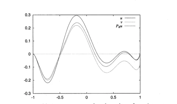
But it is rather special. We will show

an

example for the

case

$v(b)\neq 0$:

$u(x)=4(x+1)^{2}(x+ \frac{1}{2})(x-\frac{1}{5})(X-\frac{3}{5})(x-\frac{4}{5})(x-1)$for $\Omega=(-1,1)$. The graphs

of$u$, corresponding $v$ and $P_{K}u$

are

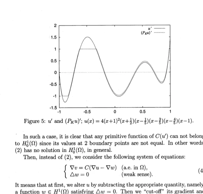
shown in Fig. 4. Also thederivatives $u’$ and

$(P_{K}u)’$ are plotted in Fig. 5.

(5)

Figure 5: $u’$ and $(P_{K}u)’;u(x)=4(X+1)2(X+ \frac{1}{2})(x-\frac{1}{5})(x-\frac{3}{5})(X-\frac{4}{5})(x-1)$ .

Insuch acase, it is clear that anyprimitive function of$C(u’)$

can

not belong

to $H_{0}^{1}(\Omega)$ since its values at 2 boundary points

are

not equal. In other words,

(2) has

no

solution in $H_{0}^{1}(\Omega)$, in general.

Then, instead of (2),

we

consider the following system of equations:

$\{$

$\nabla v=C(\nabla u-\nabla w)$ ($\mathrm{a}.\mathrm{e}$. in $\Omega$),

$\triangle w=0$ (weak sense). (4)

It

means

that at first,

we

alter$u$ by subtracting the appropriate quantity, namely,

a

function $w\in H^{1}(\Omega)\mathrm{s}\mathrm{a}\mathrm{t}\mathrm{i}\mathrm{s}\mathfrak{h}\gamma$ing $\triangle w=0$. Then we “cut-off” its gradient and

get the primitive function. If the obtained function $v$ belongs to $H_{0}^{1}(\Omega)$, then

the next theorem

assures

that $v=P_{K}u$.

Theorem 1 Let$\Omega\subset \mathbb{R}^{N}$ be a bounded domain with smooth boundary.

If

there

exists a solution $(v, w)$ in $H_{0}^{1}(\Omega)\cross H^{1}(\Omega)$ to the system

of

equations (4) with a

given parameter$u\in H_{0}^{1}(\Omega)$, then $v$ belongs to $K$ and minimizes the

functional

$J_{u}$

defined

by (1).

(Proof) It is clear that $v\in K$. Hence, it suffices to show that

$\forall f\in K$, $J_{u}(f)-J_{u}(v)\geq 0$.

Let denote $\Omega_{p}:=\{x\in\Omega;|\nabla(u-w)|>1\}$ and $\Omega_{z}:=\Omega\backslash \Omega_{p}$. Fix $f\in K$ and put $\delta:=f-v\in H_{0}^{1}(\Omega)$. For this $\delta$, we

can

easily show

(6)

since $|\nabla f|\leq 1$ and $|\nabla v|=1$ ($\mathrm{a}.\mathrm{e}$. in $\Omega_{p}$), and hence

$\nabla\delta\cdot(\nabla u-\nabla w)\leq 0$ ($\mathrm{a}.\mathrm{e}$. in $\Omega_{p}$).

On the other hand, since $\triangle w=0$ (weak

sense

in $H^{1}(\Omega)$) and $\delta\in H_{0}^{1}(\Omega)$,

$\int_{\Omega}\nabla\delta\cdot\nabla wdX=\int_{\Omega_{p}}\nabla\delta\cdot\nabla wdX+\int_{\Omega_{z}}\nabla\delta\cdot\nabla wdx=0$.

By using these facts,

we

get

$J_{u}(f)-Ju(v)= \int_{\Omega}|\nabla u-\nabla(v+\delta)|^{2}dx-\int_{\Omega}|\nabla u-\nabla v|^{2}dx$

$=$ $\int_{\Omega}|\nabla\delta|^{2}$dx–2$\int_{\Omega}\nabla\delta\cdot(\nabla u-\nabla v)dX$

$=$ $\int_{\Omega}|\nabla\delta|^{2}$dx–2$\int_{\Omega_{p}}\nabla\delta\cdot(\nabla u-\frac{\nabla u-\nabla w}{|\nabla u-\nabla w|})$ dx–2$\int_{\Omega_{z}}\nabla\delta\cdot\nabla wd_{X}$

$=$ $\int_{\Omega}|\nabla\delta|^{2}dX+2\int_{\Omega_{p}}\nabla\delta\cdot(\frac{\nabla u-\nabla w}{|\nabla u-\nabla w|}-\nabla u)dx+2\int_{\Omega_{p}}\nabla\delta\cdot\nabla wdx$

$=$ $\int_{\Omega}|\nabla\delta|^{2}dX+2\int_{\Omega_{\mathrm{p}}}(|\nabla u-\nabla w|-1-1)\nabla\delta\cdot(\nabla u-\nabla w)dX$

$\geq$ $\int_{\Omega}|\nabla\delta|^{2}dX$ $\geq$ $0$.

$\square$

3

1

dimensional

case

Theorem 1

assures

that if

one

could solve the system of equations (4) with

a

given parameter $u\in H_{0}^{1}(\Omega)$,

one

get the projection $P_{K}u$. But unfortunately,

there may not be any solution to (4) in general, except 1 dimensional

case.

In

fact, when $\Omega=(a, b)\subset \mathbb{R}^{1}(-\infty<a<b<\infty)$, the equation $w”=0$

can

be

solved such

as

$w’\equiv \mathrm{c}\mathrm{o}\mathrm{n}\mathrm{s}\mathrm{t}$.

$\mathrm{a}.\mathrm{e}$. in $(a, b)$. Hence it is sufficient to solve

$v’=c(u’-\alpha)$ ₍$\mathrm{a}.\mathrm{e}$. in $\Omega$) (5)

for $v\in H_{0}^{1}(a, b)$ and a $\in \mathbb{R}$ instead of (4). And we got an iterative solution

to (5), namely,

an

algorithm to produce the sequences $\{v_{k}\}\subset H^{1}(a, b)$ and

(7)

Algorithm I Put $\alpha_{0}:=0$ and iterate thefollowings on $k=0,1,2,$ $\cdots$ . 1.

_Define

$v_{k}\in H^{1}(a, b)\cap C([a, b])$ by using $\alpha_{k}$ such as

$v_{k}(x):= \int_{a}^{x}C(u(;\xi)-\alpha k)d\xi$ $(a\leq x\leq b)$.

2. Put $\delta_{k}:=\frac{v_{k}(b)}{b-a}$ and $\alpha_{k+1}:=\alpha_{k}+\delta_{k}$.

When $v_{k}arrow v$ in $H^{1}(a, b)$ and $\alpha_{k}arrow\alpha$ in $\mathbb{R}$

as

$karrow\infty$,

one can

expect

$v(b)=0$, i.e., $v\in H_{0}^{1}(a, b)$. If it holds, the pair of$v$ and a solves to (4). In fact,

these properties

are

assured by the following theorem.

Theorem 2 For any $u\in H_{0}^{1}(a, b)$, each sequence $\{\alpha_{k}\}$ and $\{v_{k}\}$ in

Algo-rithm Iconverges. Moreover, the limit

_{function of}

$v_{k}$ belongs to $H_{0}^{1}(a, b)$.

Theorem 2 is the direct result of following 3 lemmas. At first, we will prove

the

convergence

of $\{\alpha_{k}\}$ by showing the monotonicity and the boundedness of it.

Lemma 1 (monotonicity) In Algorithm $I$,

if

$\alpha_{1}=\delta 0:=\frac{1}{b-a}\int_{a}^{b}C(u’(\xi))d\xi>0$,

then the sequence $\{\delta_{k}\}$

satisfies

that $0\leq\delta_{k+1}\leq\delta_{k}(k=0,1,\mathit{2}, \cdots)$.

(Proof) Fix $k\in\{0,1,\mathit{2}, \cdots\}$ and

assume

$\delta_{k}\geq 0$. Let denote

$\Omega_{p}(f):=\{x\in\Omega;f(x)>1\}$, $\Omega_{n}(f):=\{x\in\Omega;f(x)<-1\}$,

$\Omega_{z}(f):=\Omega\backslash (\Omega_{p}(f)\cup\Omega_{n}(f))$,

where $\Omega=(a, b)$, and define $\Omega_{ij}$ by

$\Omega_{ij}$ $:=$ $\Omega_{i}(u’-\alpha k+1)\cap\Omega_{j}(u-\alpha_{k}’)$ $(i,j\in\{p, z, n\})$.

For brevity, wewill

use

the notations

(8)

Note that

$| \Omega|:=b-a=\sum_{i_{J}},’|\Omega_{ij}|$ and $\sum_{i,j}\omega_{ij}=1$ $(i,j\in\{p, z, n\})$,

and $|\Omega_{pz}|=|\Omega_{pn}|=|\Omega_{zn}|=0$ since $\alpha_{k+1}=\alpha_{k}+\delta_{k}\geq\alpha_{k}$

.

By using them,

we

can

write

$\delta_{k+1^{-}}\delta k=\frac{1}{|\Omega|}\sum_{i,j}\int_{\Omega_{ij}}\{C(u-\alpha k+1)’-C(u’-\alpha_{k})\}d_{X}$

$=$ $\frac{1}{|\Omega|}\{\int_{\Omega_{z\mathrm{p}}}(u’-\alpha_{k1}+-1)d_{X+}\int_{\Omega_{zz}}(-\alpha_{k}+1+\alpha k)dX$

$+ \int_{\Omega_{np}}(-2)dX+\int_{\Omega}nz(-1-u’+\alpha_{k})d_{X}\}$

$=$ $\frac{1}{|\Omega|}\int_{\Omega_{zp}}(u’-\alpha_{k1}+-1)dx-\omega_{z}z\delta k-2\omega_{np}+\frac{1}{|\Omega|}\int_{\Omega_{nz}}(-1-u’+\alpha_{k})d_{X}$

.

From the definition of $\Omega_{zp}$ and $\Omega_{nz}$, we obtain the following evaluations:

$- \min\{2, \delta_{k}\}\leq u(JX)-\alpha k+1-1\leq 0$ ($\mathrm{a}.\mathrm{e}$. $x$ in $\Omega_{zp}$),

$- \min\{\mathit{2}, \delta k\}\leq-1-u’(X)+\alpha_{k}\leq 0$ ($\mathrm{a}.\mathrm{e}$

.

$x$ in $\Omega_{nz}$).

By the estimates from above,

we

get the monotone decreasingness of $\{\delta_{k}\}$:

$\delta_{k+1}\leq(1-\omega_{z}z)\delta k-2\omega_{np}\leq\delta_{k}$.

Next,

we

will show the non-negativeness of $\{\delta_{k}\}$. By the estimates from below,

we

get

$\delta_{k+1}\geq-\min\{\mathit{2}, \delta k\}\omega_{zp}+(1-\omega_{z}z)\delta_{k}-2\omega_{np}-\min\{2,\delta_{k}\}\omega nz$

.

When $\delta_{k}\geq \mathit{2}$,

we can

deduce from this estimate

$\delta_{k+1}\geq 2(-\omega zp+1-\omega zz-\omega n\mathrm{P}-\omega_{nz})\geq 0$.

Inthe other hand, when $\delta_{k}<2$,

we can

easily show that $\omega_{np}=0$, andhence

$\delta_{k+1}\geq\delta_{k}(-\omega zp+1-\omega_{zzn}-\omega Z)\geq 0$

.

$\square$

(9)

Corollary 2 In Algorithm $I$,

if

$\alpha_{1}=\delta_{0}:=\frac{1}{b-a}\int_{a}^{b}C(u’(\xi))d\xi<0$,

satisfies

that _{$0\geq\delta_{k+1}\geq\delta_{k}(k=0,1,2, \cdots)$}.

It is obvious that $\delta_{k}=0$ implies $\delta_{k’}=0$ for all _{$k’\in\{k, k+1, k+2, \cdots\}$}.

Since $\alpha_{k}=\sum_{j=0^{1}}^{k-}\delta j$, it is easy to look that $\{\alpha_{k}\}$ is also monotone and that the

sign of$\alpha_{k}$ is “same”

as

that of$\delta_{k}$ in the

sense

considering the signof$0$ to belong

to both ofplus and minus

one.

Hence,

we

get the following.

Corollary 3 For the sequences $\{\delta_{k}\}$ and $\{\alpha_{k}\}$ generated by Algorithm $I$, it

holds that

$\alpha_{k}>0\Rightarrow\delta_{k}\geq 0$ and $\alpha_{k}<0\Rightarrow\delta_{k}\leq 0$ $(k=0,1,\mathit{2}, \cdots)$.

We

use

this property in the proof of Lemma

4.

Lemma 4 (boundedness) In Algorithm $I_{f}$ the sequence $\{\alpha_{k}\}$ is bounded

such as

$| \alpha_{k}|\leq(\frac{2}{b-a})^{1/2}||u||_{H_{0}^{1}()}a,b+1$ _{$(k=0,1,2, \cdots)$}.

(Proof) When $u=0$ in $H_{0}^{1}(a, b)$, it is clear that $\alpha_{k}=0$ for any $k\in$

$\{0,1,\mathit{2}, \cdots\}$. Then,

we

take $u\neq 0$, namely, $||u||_{H_{0}^{1}()}a,b=||u’||_{L^{2}}(a,b)>0$. And

we

will show only for the

case

$\alpha_{k}>0$ here. Almost the

same

proof works for the

case

$\alpha_{k}<0$.

For each fixed $\epsilon>0$,

assume

that

$\exists k\in \mathrm{N}$ $\mathrm{s}.\mathrm{t}$. $\alpha_{k}\geq(\frac{2+\in}{b-a})^{1/2}||u||_{H_{0}}1(a,b)+1$

.

$(*)$

Note that $\delta_{k}\geq 0$ since $\alpha_{k}>0$. Putting

$\Omega_{1}:=\{x\in\Omega;u^{J(}\backslash ^{x})-\alpha_{k}\geq-1\}$, $\Omega_{2}:=(a, b)\backslash \Omega_{1}$,

we

get the inequality

$(b-a)\delta_{k}$ $=$ $\int_{\Omega_{1}}C(u^{J}(\xi)-\alpha_{k})d\xi+\int_{\Omega_{2}}C(u(’\xi)-\alpha k)d\xi$

$(\dagger)$

(10)

where $| \Omega_{i}|:=\int_{\Omega_{i}}dx$. Since $|\Omega_{2}|=(b-a)-|\Omega_{1}|,$ $|\Omega_{1}|=0$ implies that $\delta_{k}<0$

which contradicts to the assumption $(*)$

.

Then,

we assume

$|\Omega_{1}|>0$ hereafter.

By using $(*)$ and the definition of$\Omega_{1}$,

we can

easily show that

$\xi\in\Omega_{1}\Rightarrow|u’(\xi)|2\geq(\alpha k-1)^{2}\geq\frac{2+\epsilon}{b-a}||u|J|^{2}L2(a,b)$.

Hence, it follows that

$||u’||_{L(}^{2}2a,b) \geq\int_{\Omega_{1}}|u’(\xi)|^{2}d\xi\geq\frac{2+\epsilon}{b-a}||u’||_{L(}^{2}2a,b)|\Omega_{1}|$,

and then,

$|\Omega_{2}|-|\Omega_{1}|\geq\epsilon|\Omega_{1}|$.

This and (\dagger) lead that $\delta_{k}<0$ which contradicts to $(*)$. $\square$

Lemma1 (Corollary 2) andLemma4show theconvergence of$\{\alpha_{k}\}$ generated

by Algorithm I. Then, we will show the convergence of $\{v_{k}\}$ in $H^{1}(a, b)$.

Lemma 5 For $\{\alpha_{k}\}$ and $\{v_{k}\}$ generated by Algorithm $I$, denoting

$\alpha:=\lim_{karrow\infty}\alpha_{k}$ and $v(x):= \int_{a}^{x}C(u’(\xi)-\alpha)d\xi$ $(a\leq x\leq b)$, it holds that $v_{k}arrow v(karrow\infty)$ in$H^{1}(a, b)$ and $v\in H_{0}^{1}(a, b)$.

(Proof) It is easy to see that

$\forall z_{1},$$z_{2}\in \mathbb{R}$, $|C(z_{1})-C(z2)|\leq|_{Z_{1^{-}}}z_{2}|$. By using this property and the definitions of$v$ and $v_{k}$,

we

get

$|v’(x)-v’(kX)|=|C(u’(x)-\alpha)-c(u’(x)-\alpha k)|\leq|\alpha-\alpha_{k}|$ ($\mathrm{a}.\mathrm{e}$. in $\Omega$).

Therefore, we obtain

$||v-v_{k}||_{H(\Omega}21):= \int_{a}^{b}|v(x)-v_{k}(X)|^{2}dx+\int_{a}^{b}|v’(x)-v_{k}(\prime X)|^{2}dx$

$=$ $\int_{a}^{b}|\int_{a}^{x}(v’(\xi)-v(\prime k\xi))d\xi|2dx+\int_{a}^{b}|v’(x)-v_{k}(\prime X)|^{2}dx$

$\leq$ $\int_{a}^{b}|\alpha-\alpha_{k}|^{2}(x-a)^{2}dx+\int_{a}^{b}|\alpha-\alpha_{k}|^{2}d_{X}$

(11)

and then the

convergence

$v_{k}arrow v$ in $H^{1}(a, b)$. Furthermore, since

$|v(b)-v_{k(b)|}$ $=$ $| \int_{a}^{b}(v’(X)-v’k(x))dx|$

$\leq$ $\int_{a}^{b}|v’(x)-v’k(X)|dx\leq|\alpha-\alpha_{k}|(b-a)$,

it holds that $v_{k}(b)arrow v(b)(karrow\infty)$. In the other hand, $v_{k}(b)=\delta_{k}(b-a)=(\alpha_{k+1}-\alpha_{k})(b-a)$

implies $v_{k}(b)arrow 0$, hence

we

get $v(b)=0$, namely, $v\in H_{\mathit{0}}^{1}(a, b)$. $\square$

4 Radial symmetric

case

For higher dimensional cases, the system of equations (4) may not have any

solution, in general. But, when both of domain $\Omega$ and given function

$u$

are

radial symmetric, the problem is reducible to 1 dimensional one, and

can

be

solved. In this section,

we

consider that both $\Omega$ and

$u$

are

radial symmetric.

At first, wemention about the most simple (trivial) case, namely, the domain

$\Omega$ is spherical

one:

$\Omega=\{x\in \mathbb{R}^{N};|x|<a\}$ with _$0<a<\infty$.

In this case, it is obvious that $v=P_{K}u$

can

be obtained such

as

$v(x):=- \int_{|x|}^{a}C(\tilde{u}(’\rho))d\rho$ $(x\in\Omega)$,

where $\tilde{u}$ : $\mathbb{R}arrow \mathbb{R}$ is defined by _{$\tilde{u}(|x|):=u(x)$}.

For

more

interesting case,

we

consider a ring domain:

$\Omega=\{x\in \mathbb{R}^{N};a<|x|<b\}$ with $0<a<b<\infty$

.

(6)

In this case, the system ofequations (4) can be written as

$\{$

$v_{r}=C(u_{r}-w_{r})$ ($\mathrm{a}.\mathrm{e}$. in $\Omega$), $w_{rr}+ \frac{N-1}{r}w_{r}=0$ (weak sense)

with $r:=|x|$. Since the 2nd equation of this system is solvable such

as

(12)

with arbitrary constant $\alpha$, it suffices to solve

$\tilde{v}’(r)=C(\tilde{u}’(r)-\alpha r^{1-N})$ $(\mathrm{a}.\mathrm{e}. r\in[a, b])$ (7)

for $\tilde{v}\in H_{0}^{1}(a, b)$ and $\alpha\in$ R. The equation (7) is similar to (5) and

we can

expand Algorithm I to solve it

as

followings.

Algorithm II Put $\alpha_{0}:=0$ and iterate thefollowings

for

$k=0,1,2,$$\cdots$

.

1.

_Define

$v_{k}(x)$ by using $\alpha_{k}$ such as

$v_{k}(x):= \int_{a}|x|C(\tilde{u}’(\rho)-\frac{\alpha_{k}}{\rho^{N-1}})d\rho$ $(x\in\Omega)$.

2. Put $\delta_{k}:=\frac{a^{N-1}}{b-a}\lim_{|x|arrow b}v_{k}(x)$ and $\alpha_{k+1}:=\alpha_{k}+\delta_{k}$.

This algorithm isjustified by the next theorem.

Theorem 3

_If

$\Omega$ is a ring domain such

as

(6) and $u\in H_{0}^{1}(\Omega)$ is radial

symmetric one, then $each^{-}sequenCe$

of

$\{\alpha_{k}\}$ and $\{v_{k}\}$ in Algorithm IIconverges.

The sequence $\{\alpha_{k}\}$ generated by Algorithm II also has the monotonicity and

the boundedness, and the

convergence

of $\{\alpha_{k}\}$ is direct result of them. Once

the convergence of $\{\alpha_{k}\}$

was

shown,

one can

also show the convergenceof $\{v_{k}\}$.

These lemmas written below prove Theorem

3.

Lemma 6 (monotonicity) In Algorithm II,

_if

$\alpha_{1}=\delta 0:=\frac{a^{N-1}}{b-a}\int_{a}^{b}C(\tilde{u}’(\rho))d\rho>0$,

satisfies

that $0\leq\delta_{k+1}\leq\delta_{k}(k=0,1,2, \cdots)$.

Lemma 7 (boundedness) In Algorithm II, the sequence $\{\alpha_{k}\}$ is bounded

such as

$| \alpha_{k}|\leq b^{N-1}(\frac{2}{b-a})^{1/2}||\tilde{u}’||L2(a,b)+1$ $(k=0,1,2, \cdots)$.

Lemma 8 For$\{\alpha_{k}\}$ and $\{v_{k}\}$ generated by Algorithm II, denoting

$\alpha:=\lim_{karrow\infty}\alpha_{k}$ and $v(x):= \int_{a}|x|C(\tilde{u}’(\rho)-\frac{\alpha}{\rho^{N-1}}\mathrm{I}d\rho$

$(x\in\Omega)$,

(13)

The proofs of Lemma 6,

7

and

8 are

done by almost

same

arguments

as

Lemma 1, 4 and 5, respectively, and

we

omit them here.

Finally,

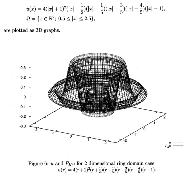
we

will show

an

example of numerical result of Algorithm II. In

Fig. 6, $u$ and $P_{K}u$ defined in 2 dimensional ring domain $\Omega$ such

as

$u(x)=4(|X|+1)^{2}(|x|+ \frac{1}{2})(|_{X}|-\frac{1}{5})(|X|-\frac{3}{5})(|X|-\frac{4}{5})(|X|-1)$, $\Omega=\{x\in \mathbb{R}2;0.5\leq|x|\leq 2.5\}$,

are

plotted

as

$3\mathrm{D}$ graphs.

Figure

6:

$u$ and $P_{K}u$ for 2 dimensional ring domain

case:

$u(r)=4(r+1)2(r+ \frac{1}{2})(r-\frac{1}{5})(r-\frac{3}{5})(r-\frac{4}{5})(r-1)$.

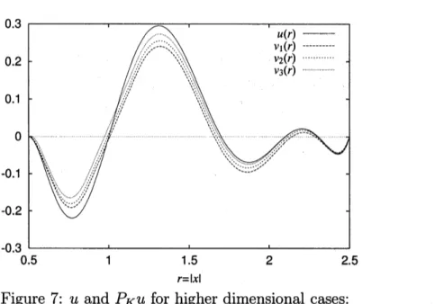
In Fig. 7, the

same

$u$and $P_{K}u$ expressed above but for 1, 2 and 3dimensional

domains are plotted

as

$r-u$ and $r-P_{K}u$ graphs. One may notice that the

differ-ence

betweenthe valuesof$u$ and those of$P_{K}u$ israther uniform in 1 dimensional

case.

But in

a

higher dimensional case, the difference between the values of $u$

(14)

$r=|X\mathrm{I}$

Figure

7:

$u$ and $P_{K}u$ for higher dimensional

cases:

$v_{n} \mathrm{d}\mathrm{e}\mathrm{n}u(r)=4\mathrm{o}\mathrm{t}\mathrm{e}\mathrm{s}P_{K}^{+1}(ru)^{2}(r\mathrm{f}_{\mathrm{o}\mathrm{r}n}\dim+\frac{1}{2})(r-\frac{1}{5})(r-\frac{3}{51})\mathrm{e}\mathrm{n}\mathrm{S}\mathrm{i}\mathrm{o}\mathrm{n}\mathrm{a}\mathrm{C}\mathrm{a}\mathrm{s}\mathrm{e}(r-\frac{4}{5}.)(r-1)$ ;