Dynamical systems of
Certain
$\mathrm{n}\mathrm{o}\mathrm{n}-\mathrm{h}\mathrm{o}1_{\mathrm{o}\mathrm{m}_{\check{i}}\mathrm{o}}\mathrm{r}\mathrm{P}\mathrm{h}\mathrm{i}\mathrm{c}$maps
東海大理学部内村桂輔 (Keisuke Uchimura)
1
Introduction
Complex dynamical systems given by quadratic polynomials
$f_{c}(z)=z2+C$
havemany well-known important analytic andgeometricproperties. When$c=-2$, $f_{-2}(Z)$
has relation to a Chebyshev polynomial. The Julia set of $f_{-2}(Z)$ is the interval [-2, 2].
For any $z$ in [-2, 2], we set
$z=\psi(\theta)=e^{\pi\theta i}+e^{-}\pi\theta i$,
where $\psi$ is afunction from $\mathrm{R}$ to [-2, 2]. Clearly
$\psi(\theta)=\psi(\theta+2)=\psi(2-\theta)$.
Then we introduce an equivalence $\mathrm{r}\mathrm{e}\mathrm{l}\mathrm{a}\mathrm{t}\mathrm{i}\mathrm{o}\mathrm{n}\sim \mathrm{g}\mathrm{e}\mathrm{n}\mathrm{e}\mathrm{r}\mathrm{a}\mathrm{t}\mathrm{e}\mathrm{d}$by $\theta\sim\theta+2$, $\theta\sim 2-\theta$. Hence
we have
an
induced map$\psi$
:
$\mathrm{R}/\simarrow[-2,2]$.Let $t$ be a transformation on $\mathrm{R}/$ \sim deflned by $t(\theta)=2\theta$. Then two dynamical systems
$\mathrm{t}1^{-2,2}],$$f-2\}$ and $\{\mathrm{R}/\sim, t\}$ are topological conjugate and the induced map $\psi$ is a
topological conjugacy. $\{\mathrm{R}/\sim, t\}$ is equivalent to the dynamical system given by a tent
map on $[0,1]$.
Two-dimensinal extension of thesedynamical systems is considered. Let
$z=\Psi(\sigma, \tau)=e+\pi\sigma e^{-}+e2i2\pi\tau i2\pi(\mathcal{T}-\sigma)i$.
Then $\Psi$ maps $\mathrm{R}^{2}$ to asubset $\mathrm{S}$ in the complex plane C. Clearly
$\Psi(\sigma, \tau)=\Psi(\sigma+1, \tau)=\Psi(\sigma, \tau+1)$ .
Then $\Psi$ may be considered as a map from two-dimensional tours $T^{2}$ to $S$
.
Further $\Psi(\sigma, \tau)=\Psi(\sigma, \sigma-\mathcal{T})=$ 申$(-\sigma+\tau, \tau)=\Psi(1-\mathcal{T}, 1-\sigma)$.Then we introduce an equivalence $\mathrm{r}\mathrm{e}\mathrm{l}\mathrm{a}\mathrm{t}\mathrm{i}\mathrm{o}\mathrm{n}\sim \mathrm{o}\mathrm{n}T^{2}$defined by
$(\sigma, \tau)\sim(\sigma, \sigma-\tau)\sim(-\sigma+\tau, \tau)\sim(1-\tau, 1-\sigma)$ . (1.1)
Hence we have
an
induced map$\Psi$
:
$T^{2}/\simarrow S$.
An extension of $f_{-2}(Z)$ is
a
map:
$F_{2}(z)=z^{2}-2\overline{Z}$.
Then
$F_{2}(\Psi(\sigma, \tau))=\Psi(2\sigma, 2\tau)$
.
Let $d$ be adouble angle map of $T^{2}/\sim \mathrm{o}\mathrm{n}\mathrm{t}\mathrm{o}$ itself. That is,
$d(\sigma, \mathcal{T})=(2\sigma, 2\mathcal{T})$
.
Then $\{S, F_{2}\}$ and $\{T^{2}/\sim, d\}$ are topological conjugate. Hence $F_{2}(z)$ is a two-dimension
extension of$f_{-2}(Z)$
.
Uchimura [1996] shows that $\{S, F_{2}\}$ is chaotic.2
The
dynamics
of
$F_{2}$We study the dynamical
system
given by$F_{2}(z)=$. $z2-2\overline{Z}$. (2.1)
We shall show that $F_{2}$ partition the complex plane $\mathrm{C}$ into two sets.
One
is a closed$\mathrm{d}_{\mathrm{o}\mathrm{n}\mathrm{l}\mathrm{a}}\mathrm{i}\mathrm{n}S$ and the other is its complement. The dynamics of $\mathrm{A}I7_{2}$
on
$\mathrm{S}$ is chastic and thecomplement of $S$ is the $\mathrm{b}\mathrm{a}s$in of
$\infty$ of $F_{2}$.
Since $F_{2}(z)$ is not holomorphic, we regard the function $F_{2}$ as a function of two real
variables. That is,
$F_{2}((x, y))=(x^{2}-y^{2}-2X,2_{X}y+2y)$. (2.2)
Here $z=x+iy$. The
Jacobian
determinant of $F_{2}$ is $4x^{2}+4y^{2}-4$.
So
the set ofcriticalvalues is an algebraic curve ofthe fourth degree which is known as Steiner’s hypocycloid.
It takes the form
$(x^{2}+y^{2}+9)^{2}+8(-x^{3}+3xy^{2})-108=0$. (2.3)
Let $S$ be aclosedregion bounded bySteiner’s hypocycloid (2.3). See [Koornwinder, 1974].
We shall show that the function $F_{2}(z)$ restricted to the set $S$ is a finiteto-one factor
of the algebraic endomorphism of the torus given by the matrix
Then the point $(\sigma, \tau)$ is regarded as a point in the torus $T\simeq \mathrm{R}^{2}/\mathrm{Z}^{2}$. From Then, we have
a torus endomorphism $l$ on $T$ given by
$(\sigma, \tau)$ is equivalent tothe points $(-\sigma+\tau, \tau),$ $(\sigma, \sigma-\tau)$ and $(1-\tau, 1-\sigma)$
.
$\mathrm{T}$,hat
is to say,we have to consider an equivalence relation given by
$(\sigma, \tau)\sim(-\sigma+\tau, \mathcal{T}),$ $(\sigma, \tau)\sim(\sigma, \sigma-\tau),$ $(\sigma, \tau)\sim(1-.\mathcal{T}, 1-\sigma).\cdot.$
.
(2.5)Let $R=T/\sim$.
The set $R$ is regarded as a closed region bounded by a regular triangle $OAB$ with
$O=(\mathrm{O}, 0),$ $A=( \frac{1}{2}, \frac{-1}{2\sqrt{3}}),$ $B=( \frac{1}{2}, \frac{1}{2\sqrt{3}})$, in the $(\mathrm{s},\mathrm{t})$-plane, where
$s=(\sigma+\tau)/2,$ $t=\sqrt{3}(\sigma-\tau)/2$
.
Nowwe consider the symbolic dynamics. For any point$x\in R$, we define
the.
itinerary$h(x)$ by the rule
$h(x)=(s_{0}s_{12}s\ldots)$
where $s_{j}=k$ if and only if $d^{j}(x)\in\triangle(k),$ $(k=0,1,2,3)$. Here $\triangle(0)=\triangle DEF,$ $\triangle(1)=$
$\triangle OEF,$ $\triangle(2)=\triangle ADF,$ $\triangle(3)=\triangle BED$, where $D,$$E$ and $F$ are the midpoints of
AB,$OB$ and $OA$, respectively.
Set
$\Sigma_{4}=$
{
$(s0s1s2\cdots)|s_{j}=0,1,2$or3}.
We introduce
an
equivalence $\mathrm{r}\mathrm{e}\mathrm{l}\mathrm{a}\mathrm{t}\mathrm{i}\mathrm{o}\mathrm{n}\sim \mathrm{o}\mathrm{n}\Sigma_{4}$ which is defined by$(w_{1}0w_{2})\sim(w_{1}2w_{2})$, for$w_{1}\in\{0,1,2,3\}*,$ $(w_{2})\in h(OA)$,
($w_{1,-}\mathrm{o}_{w_{2})}\sim(w_{1}3w_{2})$, for$w_{1}\in\{0,1,2,3\}*,$ $(w_{2})\in h(OB)$, $!.\mathrm{t}$
$(w_{12}0w)\sim(w_{1}1w_{2})$, for$w_{1}\in \mathrm{t}0,1,2,3\}^{*},$ $(w_{2})\in h(AB)$
.
Let $\Sigma’$ denote the quotient $\Sigma_{4}/\sim$. Note that
$\sigma$ is naturally defined on $\Sigma’$. That is,
$\sigma[(s_{0^{S_{1}\ldots s}}n\cdots)]=[(S_{1}\ldots s_{l},\ldots)]$.
Clearly $\sigma$ is well-defined.
Theorem 2.1. The mapping $\tilde{h}$
: $Rarrow\Sigma’$ is a bijection and it makes the following
diagram commutative: $d$ $R$ $R$ $\tilde{h}\}\Sigma$ ’ $\Sigma\downarrow\tilde{h,}$ $\sigma$
Let $\Gamma$ be a Sierpinsky gasket
$\mathrm{w}\backslash$hose outermost triangle is $OAB$
.
Then itcan
be easilyseen
that$d(\Gamma)=\Gamma$
.
Let
$\Sigma"=$
{
$[(s0S1\cdots Sn\cdots)]$ $|s_{i}\in\{1,2,3\}$,
for all $i$}.
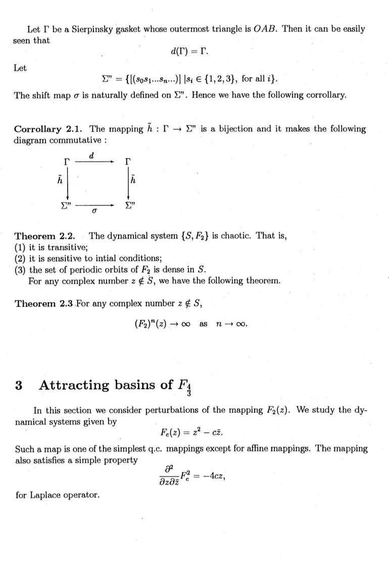
The shift map $\sigma$ is naturally defined on $\Sigma$”. Hence we have the following corrollary.
Corrollary 2.1. The mapping $\tilde{h}$
:
$\Gammaarrow\Sigma$” is a bijection and it makes the followingdiagram commutative: $d$ $\Gamma$ $\Gamma$ $\tilde{h}\}\Sigma$ ” $\Sigma \mathrm{I}^{\tilde{h}},$ , $\sigma$
Theorem 2.2. The dynamical system $\{S, F_{2}\}$ is chaotic. That is,
(1) it is transitive;
(2) it is sensitive to intial conditions;
(3) the set of periodic orbits of $F_{2}$ is dense in $S$.
For any complex number $z\not\in\grave{S}$, we have the following theorem.
Theorem 23For
any
complex number $z\not\in S$,$(F_{2})^{n}(z)arrow\infty$ as $narrow\infty$
.
3
Attracting
basins of
$F_{4,3}$In this section weconsider perturbations of the mapping $F_{2}(z)$
.
We study thedy-namical systems given by
$F_{c}(Z)=z-2C\overline{Z}$.
Such
a
map isone
of thesimplest $\mathrm{q}.\mathrm{c}$.
mappings except for affine mappings. The mappingalso $\mathrm{S}\mathrm{a}\mathrm{t}\mathrm{i}\mathrm{S}\mathrm{p}_{\mathrm{e}\mathrm{s}}$ asimple property
$\frac{\partial^{2}}{\partial z\partial\overline{z}}F_{c}^{2}=-4Cz$,
First we note that tllere are four fixed points and $12_{\mathrm{P}^{\mathrm{e}\mathrm{r}}}.\mathrm{i}\mathrm{o}\mathrm{d}\mathrm{i}\mathrm{C}$ points of prime period
2 which are listed in $\mathrm{U}\mathrm{c}\mathrm{h}\mathrm{i}\mathrm{m}\mathrm{u}\mathrm{r}\mathrm{a}[1977]$.
We study the dynamics of $F_{c}(z)$ when $c= \frac{4}{3}$
.
The value $c= \frac{4}{3}$ is a special value inthe
sense
that all attractive fixed points and attractive periodic points ofp.eriod
2 lieon
a critical set. We will study attractive basins of$F_{\frac{4}{3}}$
.
When $c \cdot=\frac{4}{3}$, two attracting fixed points $P_{\langle 1)}^{2}$ and $P_{(1)}^{3}$ are written as
$P_{11}^{2}=)- \frac{1}{6}+i\sqrt{\frac{5}{12}}$
$F_{(1)}^{3}=\overline{P_{(}21)}$.
There are four attracting periodic points of period 2 which are written as
$P^{2}=\omega P^{2}P^{3}=\omega(2)(1)’(2)(1)2P2$
$P_{(2)}^{4}=\omega P_{(}^{3}P^{5}=1)’(2)\omega P_{()}231$.
Critical
points of $F_{\frac{4}{3}}(z)$ are thezeros
ofJacobian
determinent of$F_{\frac{4}{3}}$.
Then critical set of$F_{\frac{4}{3}}(z)$ is equal to a circle $\{z;2|z|=\frac{4}{3}\}$. Note that the attracting periodic points $P_{(1)}^{2}$, $P_{(1)’(2}^{3}P^{2})’ P_{(2)’(2}^{3}P^{4})’ P_{(2)}^{5}$ lie on the circle. Set
$A=( \frac{4}{3},0)$, $‘ f \mathit{3}=(-\frac{2}{3}, \frac{2\sqrt{3}}{3})$ and $C=(- \frac{2}{3}, -\frac{2\sqrt{3}}{3})$.
Theorem 3.1. The interiors of the triangular regions $\triangle OBD$ and $\triangle OCF$ are the
im-mediate $\mathrm{b}\mathrm{a}s$ins of Pxed points
$P_{(1)}^{2}$ and $P_{(1)}^{3}$
.
The interiors of $\triangle OBE$ and $\triangle OAD$are
immediate $\mathrm{b}\mathrm{a}s$ins of periodic points
$P_{(2)}^{4}$ and $P_{(2)}^{5}$. The interiors of $\triangle OCE$. and $\triangle OAF$
are immediate basin ofperiodic points $P_{(2)}^{2}$ and $P_{(2)}^{3}$
.
By the symmetry we know that to prove Theorem 3.1 it suffices to prove the following
proposition.
Proposition 3.1. Let $z$ be any interior point of $\triangle OBD$. Then
$(F_{\frac{4}{3}})^{n}(z)$
.
$arrow P_{(1)}^{2}$ $(narrow\infty)$
.
References
Koornwinder, T. H. [1974] ”Orthogonal polynimials in two variables $\mathrm{w}\mathrm{h}\mathrm{i}\mathrm{c}\mathrm{h}_{t}|\mathrm{a}\mathrm{r}\mathrm{e}$
eigenfunctions
of twoalgebraically
independent partial differential operators III IV”,Indag. Math. 36,
357-381.
Uchimura, K. [1996] ” The dynamical systems associated with Chebyshev polynomials
in two variables”, Int.
J.
Bifurcation
and Chaos, 6, $12\mathrm{B},$ $26l$1-2618.
Uchimura, K. [1997] ”Attracting basins of certain non-holomorphic map”,