The Nonstationary Infinite Horizon Production-inventory Problem with Uncertain Capacity and Uncertain Demand (Mathematical Decision Making under uncertainty and ambiguity)

The

Nonstationary

lnfinite

Horizon

Production-inventory

Problem

with

Uncertain

Capacity and

Uncertain

Demand

Department of Industrial Engineering and Management, Tokyo Institute of Technology,

TetsuoIida

東京工業大学経営工学専攻 飯田哲夫

1

Introduction

In this paper we consider

a

non-stationary periodic review dynamic production-inventory

model with uncertain production capacity and uncertain demand. The demands occur

inde-pendently,but they

are

not necessarily identically distributed. Also, themaximumproduction

capacityvaries stochastically. This is because of uncertainties in production processes. for

in-stance, unexpected breakdown and unplanned maintenance (Ciarallo, Akella and $\mathrm{M}\mathrm{o}\mathrm{r}\mathrm{t}\mathrm{o}\mathrm{n}[3]$).

Therefore, if the realized production capacity is below the planned production quantity, only

part ofit can be produced.

The non-stationarystochasticperiodicreviewinventorymodels havebeenstudiedbynany

researchers; see$\mathrm{K}\mathrm{a}\mathrm{r}\mathrm{l}\mathrm{i}\mathrm{n}[11,12],$ $\mathrm{v}\mathrm{e}\mathrm{i}\mathrm{n}\mathrm{o}\mathrm{t}\mathrm{t}[16, ?],$ $\mathrm{M}\mathrm{o}\mathrm{r}\mathrm{t}\mathrm{o}\mathrm{n}[14],$$\mathrm{Z}\mathrm{i}_{\mathrm{P}}\mathrm{k}\mathrm{i}\mathrm{n}[19]$, Morton and$\mathrm{P}\mathrm{e}\mathrm{n}\mathrm{t}\mathrm{i}\mathrm{C}\mathrm{o}[15]$,

and$\mathrm{I}\mathrm{i}\mathrm{d}\mathrm{a}[9]$

.

However all of theses literature do not consider the productioncapacityconstraint.

The stationary models with the production capacity constrainthave been studied

(Feder-gruen and $\mathrm{Z}\mathrm{i}\mathrm{p}\mathrm{k}\mathrm{i}\mathrm{n}[4,5]$, Ciarallo, Akella and $\mathrm{M}\mathrm{o}\mathrm{r}\mathrm{t}\mathrm{o}\mathrm{n}[3],$ $\mathrm{G}\ddot{\mathrm{u}}1\mathrm{l}\ddot{\mathrm{u}}[8])$

.

A multi-stage model with

the production capacity constraint has been studied (Glasserman and $\mathrm{T}\mathrm{a}\mathrm{y}\mathrm{u}\mathrm{r}[6,7]$). A

peri-odic(cyclic) demand model with the productioncapacity constraint is studiedin Kapu\’{s}citski

and $\mathrm{T}\mathrm{a}\mathrm{y}\mathrm{u}\mathrm{r}[13]$

.

The stationary models with random yields have been studied (Yano and

$\overline{\mathrm{L}}\mathrm{e}\mathrm{e}[18]$, Wang and $\mathrm{G}\mathrm{e}\mathrm{r}\mathrm{c}\mathrm{h}\mathrm{a}\mathrm{k}[17])$

.

It is known that myopic (or

near

myopic) policies are nearly optimal for the inventory

problems without the production capacity. However, it has not been known whether the

near myopic policies are still nearly optimal for the production-inventory problems with the

production capacity. In this paperweshow that the similar result holds for theproblemswith

the productioncapacity.

We considera single-stage non-stationary production-inventory model withuncertain

pro-duction capacity and uncertain demand. Theobjective ofour model is to minimize thetotal

discounted expected costs which include production, inventory holding and penalty costs.

Production, inventory holding and penalty costs

are

assumed to be linear respectively. We

deal with both finite horizon problems and infinite horizon problems for which order up-to

(or base-stock, critical number) policies are optimal, and obtain upper and lower bounds of

optimal order up-to levels. Furthermore

we

show that for an infinite horizon problem the

upper and the lower bounds of optimal order up-to levels for the finite horizon counterparts

convergerespectively asthe plaming horizons considered become longer. Furthermore, under

mild conditions the differences between theupperand the lower bounds of optimal order up-to

We first formulate the finite horizonproblem as adynamic programalong standard steps,

and then introduce

a new

problem which is equivalent to the original problem with respect

to the optimal expected cost and the optimal ordering policies. Then we obtain upper and

lower bounds of the optimal order up-to levels for the finite horizon problem. For the infinite

horizon problem, the convergence results ofthe upper and the lower bounds of the optimal

order up-tolevelsforthe finite horizon counterpartsareshown. Numerical examples illustrate

computation of the bounds and

convergence.

The paper is organized

as

follows. Section 2 presents the problem considered in this

paper and introduce anequivalent problem. Section 3 explores the infinite horizon problem:

we

develop upper and lower bounds of optimal order up-to levels and show the convergence

results. Section 4 presents numerical examples. Section 5 concludes this

paper:

All proofs of propositions and lemmas in this paper are shown in [10].

2

Problem Formulation

We consider

a

periodicreviewdynamic production-inventory model with uncertainproduction

capacity and uncertaindemand. The demands and the production capacities are assumed to

be independent but not necessarily be identical. Leadtime is

zero

and unsatisfied demands

are

backlogged. The objective of the problem is to minimize the total discounted expected

costs which include three types of costs: production, inventory holding and backlog penalty

costs. The costs

are

assumed to be linear respectively.

The activities take place in the following manner: at the beginning of a period a new

ordering decision ismade, duringtheperiodtheproductioncapacity realizes and the customer

demand occurs, and at the end of the period inventory holding and backlog penalty costs

are

charged.

We define

$Z_{t}$ : customer demand at period $t$,

$Q_{t}(z),$ $q_{t}(Z)$

:

cumulative distribution and density functions for $Z_{t}$,

$A_{t}$ : $\mathrm{p}\mathrm{r}\mathrm{o}\mathrm{d}\mathrm{u}\mathrm{C}\mathrm{t}\mathrm{i}_{\dot{\mathrm{O}}}\mathrm{n}$ capacity at period $t$,

$F_{t}(a),$ $f_{t}(a)$ : cumulative distribution and density functions for $A_{t}$,

$x_{t}$

:

inventory position at the beginning of period$t$ before ordering,

$u_{t}$ : planned production quantity at period $t$,

$c_{t},$ $h_{t,pt}$ : unit production, hol,ding and penalty costs at period $t(h_{t},$ $p_{t}>0,$ $c_{t}\geq 0$ and $p_{t}>c_{t})$

.

We

assume

that the unit holding, penalty and production costs are bounded, that

is, $p_{t}<p<\infty,$ $h_{t}<h<\infty$ and $0\leq\underline{c}<c_{t}<\overline{c}<\infty$ for all $t$

.

2.1

Dynamic

Programming Formulation

We first consider the expected one-period cost. The production cost is determined by the

actual production quantity which is limited by the production capacity $A_{t}$

.

If the planned

production quantityis$u_{t}$and the realized productioncapacityis$a_{t}$, then the actualproduction

quantity is $\min$

{

$u_{t}$

,

at}.

The inventory holding and backlog penalty costs are determined by

the inventory position at the end of the period whichdepends

on

therealized customer demand

$Z_{t}$

.

Thus the one-period expected cost $g_{t}(x, u)$

,

wherethe inventory position at thebeginning

of period $t$before ordering is _$x$ and the planned production quantity is _$u$, is

as

follows,

For an $n$-period problem, we minimize the total discounted expected cost. Let $\alpha<1$ be

the discount factor perperiod. Theperiods are numbered 1, 2,

...

,$n$

.

Let $G_{t,n}(x)$ denote the

total discounted expected cost from period $t$ through$n$ using optimal policies, given that the

inventory position at the beginning ofperiod $t$ before ordering is _$x$

.

Then, _{$G_{t,n}(x)$} satisfies

the following recursive equation,

$G_{t,n}(x)= \min_{u\geq 0}\{gt(x, u)+\alpha EG_{t+1,n}(X+\min\{u, A_{t}\}-z_{t})\}$, for $t=1,2,$$\ldots$ ,$n$,

where $G_{n+1,n}(X)\equiv 0$. In the above recursive equation the expectation is taken with respect

to the random variables $A_{t}$ and $Z_{t}$

.

We shall hereafterassume that all relevant functions are

differentiable. We define

$H_{t,n}(x, u)$ $=$ $g_{t}(x, u)+ \alpha EG_{t+1},n(X+\min\{u, A_{t}\}-^{z}t)$ (1) $=$ $g_{t}(x, u)+ \alpha\int_{0}^{u}\int_{0}^{\infty}ct+1,n(x+a-Z)ft(a)qt(z)dadz$

$+ \alpha(1-F(u))\int_{0}^{\infty}G_{t}+1,n(X+u-z)q_{t}(z)d_{Z}$

.

Nowwe denote the solutionof the following equation by $x_{t,n}^{*}$,

$(h_{t}+p_{t})Q_{t}(X)+ \alpha\int_{0}^{\infty}G_{t1}’(x-Z)dQ_{t(}Z)+,n-(pt-_{C}t)=0$,

and define abase-stock ordering policy $u_{t,n}^{*}(x)$ using $x_{t,n}^{*}$ as follows,

$u_{t,n}^{*}(_{X})=\{$

$x_{t,n}^{*}-x$ if $x\leq x_{t,n}^{*}$,

$0$ if _{$x>x_{t,n}^{*}$}

.

Then thefollowing proposition$\mathrm{h}\mathrm{o}\mathrm{l}\mathrm{d}_{\mathrm{S}}$(Ciarallo, Akella and

$\mathrm{M}\mathrm{o}\mathrm{r}\mathrm{t}\mathrm{o}\mathrm{n}[3]$, Wang and$\mathrm{G}\mathrm{e}\mathrm{r}\mathrm{c}\mathrm{h}\mathrm{a}\mathrm{k}[17]$).

Proposition 1 1. $G_{t,n}(x)$ is convex.

2. $G_{t,n}(x)=\{$ $H_{t,n}(x, u_{t}^{*},(nx))$ when

$x\leq x_{t,n}^{*}$, $H_{t,n}(x, \mathrm{o})$ when $x>x_{t,n}^{*}$

.

3. The base-stock policy $u_{t,n}^{*}(x)$ minimizes (1).

2.2

An Equivalent Problem

We consider aproblem equivalent to the original problem defined in the previous subsection.

Inthe original problem the available production capacity realizes after ordering, thereforewe

have to make a production order considering the uncertainty ofthe production capacity. We

here consideraproblem in which the availableproduction capacity realizesbefore ordering

so

that

we can

make

a

production order with the deterministic production capacity constraint.

We will find that this problem is equivalent to the originalone with respect to both optimal

ordering policies and optimalexpected costs, and as aresult of this modification the analysis

of the problem becomes simpler than that of the originalone. We denote the original problem

by Pl and the new one by P2.

In problem P2 the activities in

a

period take place in the following

manner:

at the

at the end of the period penalty and holding costs are

charged.

We denote the inventory position after ordering by $y_{t}$

.

Since the production capacity is

realized before ordering, we candetermine $y_{t}$ explicitly whenwe make

an

order. We consider

the expected one-periodcostwhere theinventoryposition at the beginning of the period after

ordering is$y(y=x+u)$

.

Let

$L_{t}(y)=E[h_{t}(y-zt)++pt(y-Z_{t})-]$.

Note that $L_{t}(y)$ is a convexfunction. Then the expected one-period cost where the inventory

positionat the beginning of the period after ordering is $y$ is $c_{t}(y-X_{t})+L_{t}(y)$

.

Nextwe consideran$n$-period problem. Since the ordering decision in P2 is limited by the

realized production capacity $a_{t}$,

we

consider

a

pair of the inventory position at the beginning

ofa period before ordering and the realized production capacity

as a

state, that is, $(x_{t}, a_{t})$

.

Let$I_{t,n}(x, a)$ denote the total discountedexpectedcost from period $t$ through_$n$ usingoptimal

policies, given that the inventory position at the beginning ofperiod $t$ before ordering is _$x$

and the realized production capacity in period $t$ is $a$

.

We also define

$I_{t,n}(x)=EI_{t,n}(x, A_{t})$. (2)

Then $I_{t,n}(x, a)$ satisfies the followingrecursive equation,

$I_{t,n}(x, a)= \min_{x\leq y\leq x+a}\{Ct(y-x)+L_{t}(y)+\alpha EI_{t+1,n}(y-Z_{t})\}$, (3)

where $I_{n+1,n+1()}x\equiv 0$

.

We define additional functions $J_{t,n}$ as follows,

$J_{t,n}(y)=C_{ty+}Lt(y)+\alpha EIt+1,n(y-Z_{t})$

.

Then $I_{t,n}(x, a)=-c_{t}x+ \min_{x\leq y\leq t,n}x+aJ(y)$, and the following proposition holds.

Proposition 2 $J_{t,n}(y)$ is convex.

From the convexity of$J_{t,n}(y)$ an order up-topolicy is optimal. We call$y_{t,n}^{*}$ optimal order

up-to level. It is shown in the proof that $y_{t,n}^{*}$ solves the following equation,

$J_{t,n}’(y)\equiv(h_{t}+p_{t}).Qt(y)-(pt-c_{t})+\alpha EI_{t1,n}’(+y-Zt)=0$

.

This

means

that the optimal order up-to levels are same for all$a$.

Next we come to the main result of this section. The following proposition allows us to

investigate problem P2 instead ofproblem Pl.

Proposition 3 Problems$P1$ and$P2$ are equivalentwith respectto both the optimal ordering

policies and the optimal expected costs.

In order to derive upper and lower bounds of the optimal order up-to levels in the next

section, we now make a cost transformation, whichwas used in Morton and $\mathrm{P}\mathrm{e}\mathrm{n}\mathrm{t}\mathrm{i}_{\mathrm{C}\mathrm{O}}[15]$

.

Let

$\tilde{I}_{t,n}(x, a)=c_{t}x+I_{t,n}(x, a)$ and$\tilde{I}_{t,n}(x)=c_{t}x+I_{t,n}(x)$

.

Then

we

obtainthe followingrecursive

equations for $\tilde{I}_{t,n}(x,a)$ and $\tilde{I}_{t,n}(x)$,

and

$\tilde{I}_{t,n}(x, a)=\min_{x\leq y\leq x+a}\{\tilde{L}_{t}(y)+\alpha E\tilde{I}_{t1,n}+(y-^{z_{t})}\}$ (5)

where transformed

one

period cost function $\tilde{L}_{t}$ and cost parameters are defined as follows,

$\tilde{L}_{t}(y)=\tilde{h}_{t}E(y-^{z_{t})}++\tilde{p}_{t}E(y-z_{t})-+c_{t}E[z_{t}]$

and

$\tilde{h}_{t}=h_{t}+c_{t}-\alpha C_{t1}+$ and $\tilde{p}_{t}=p_{t}-c_{t}+\alpha c_{t+1}$

.

Note that equations (4) and (5) are identical to equations (2) and (3). Therefore optimal

order up-to levels $y_{t,n}^{*}$

are

same. We define additional functions $\tilde{J}_{t,n}(y)$

as

follows,

$\tilde{J}_{t,n}(y)=\tilde{L}_{t}(y)+\alpha E\tilde{I}_{t}+1,n(y-z_{t})$

.

Also, let $\tilde{h}=h+\overline{c}-\alpha\underline{\mathrm{c}}$and

$\tilde{p}=p-\underline{\mathrm{c}}+\alpha\overline{c}$. Then$\tilde{p}_{t}<\tilde{p}$ and $\tilde{h}_{t}<\tilde{h}$

.

3

The Infinite

Horizon

Problem

3.1 Upper

and Lower

Bounds

of

the Optimal Order Up-to

Levels

We first consider upper and lower bounds of the optimal order up-to levels for

an

n-period

problem. We providealemma which shows monotonicity of derivatives of the optimal expected

costsand the optimal order up-to levels. The shorthand$f_{\star^{1}}$is used to meanthat the function

$f$ is everywhere decreased, and $f\uparrow \mathrm{i}\mathrm{s}$ similar.

Lemma 4 $\tilde{J}_{t,n}’\downarrow\Rightarrow\tilde{I}_{t,n}’\downarrow$, $y_{t,n}^{*}\uparrow and\tilde{J}_{t-}^{J}\downarrow 1,n$.

All results remain true if all

arrows are

inverted. Recall that $-(\tilde{p}-\alpha\underline{\mathrm{c}})\leq\tilde{J}_{n,n}’(y)\leq\tilde{h}+\alpha\overline{c}$

.

We

now

define

$\tilde{I}_{n+1,n}^{U}(x)\equiv-\frac{\tilde{p}x}{1-\alpha}$ and $\tilde{I}_{n+1,n}^{L}(x)\equiv\frac{\tilde{h}x}{1-\alpha}$.

Let$\tilde{I}_{t,n}^{U}$and$\tilde{I}_{t,n}^{L}$ denote the corresponding additional functions derived from$\tilde{I}_{n+1,n}^{U}$ and$\tilde{I}_{n+1,n}^{L}$,

respectively. Similarly

we

define $\tilde{J}_{t,n}^{U},\tilde{J}_{t,n}^{L},$ $y_{t,n}^{U*}$ and $y_{t,n}^{L*}$. Then the folowing proposition is

shown byusing Lemma 4.

Proposition 5 1. $\tilde{J}_{t,n}^{U\prime}(y)\leq\tilde{J}_{t,n}^{U;}(+1y)$

for

all$y$

.

2. $\tilde{I}_{t,n}^{U/}(X)\leq\tilde{I}_{t,n}^{U\prime}+1(x)$

for

all$x$

.

3. $y_{t,n+1}^{U}*\leq y_{t,n}^{U*}$

.

The results for the lower bounds also hold similarly. Thenwe can define

$\lim_{narrow\infty}y_{t},nU*=y_{t}^{U*}$ and $\lim_{narrow\infty}y^{L*}t,n=y^{L*}t$

’

since a bounded monotonic sequence converges to a point. Thus from proposition 5 the

Proposition 6 For any and$t<n$

.

Remark The inventory problem considered here

can

be formulated

as

a

non-homogeneous

Markov decision process. $\cdot$

Under the conditions that the demands

are

integral, the

means

of the demands

are

bounded from above and the inventory position is limited, it is shown

from the theory of non-homogeneous Markov decision processes that

a

set ofoptimalordering

policies foran infinite horizonproblem includes the limiting policy of theoptimalpolicies for

the finite horizon counterparts (Bes and $\mathrm{S}\mathrm{e}\mathrm{t}\mathrm{h}\mathrm{i}[2]$ and Bean, Smith and $\mathrm{L}\mathrm{a}\mathrm{s}\mathrm{S}\mathrm{e}\mathrm{r}\mathrm{r}\mathrm{e}[1]$).

Hereafter

we

consider the limiting policy of the optimal policies for the finite horizon

counterparts as

the.optimal

policy for the infinite horizon problem.

3.2

The

Difference

between

the Upper and the Lower Bounds

In this subsection we investigate the conditions under which a sequence of the differences

between the upper and the lower bounds of the optimal order up-to levels for the finite

horizon counterparts converges to

zero.

We first consider the relations among the second

derivatives of$\tilde{L}_{t},\tilde{J}_{t,n},\tilde{J}_{t,n}^{U}$ and so on. Let $0 \leq m_{t}\equiv\inf_{y}\tilde{L}_{t}^{\prime/}(y)$

.

and

$\triangle\tilde{J}_{t}’\equiv\tilde{J}_{t}^{L}’-\tilde{J}_{t}U’$

.

Similarly, $\Delta\tilde{I}_{t}’,$ $\triangle y_{t}^{*}$ and

so

on are defined. Next, we show the results for the relation among

$m_{t},$ $\triangle\tilde{J}_{t,n}’$ and

so

on.

Lemma 7 1. $\Delta\tilde{I}_{t,n}’(X)\leq\max_{y}\Delta\tilde{J}_{t}’,n(y)$

.

2. $m_{t} \triangle y_{t}^{*}\leq\max_{y}\Delta\tilde{J}_{t}’,(ny)$

.

Then thefollowing proposition isshown by using Lemma

7.

Proposition 8 $\triangle\tilde{J}_{t,n}’(y)\leq\alpha^{n-t+1}(\tilde{h}+\tilde{p})/(1-\alpha)$ .

Cororally 9

_If

$m_{t}>0,$ $\triangle y_{t,n}^{*}$ converges to zero as $narrow\infty$

.

The convergence rate of $\triangle y_{t,n}^{*}$ to zero is $O(\alpha^{n-t+1})$. Therefore we may expect that the

convergence is rapid for most problems. In the next section

we

investigate the speed of the

convergence with numerical examples.

4

Numerical

E.xamples

In thissection we illustrate the upper and the lower bounds of the optimal order up-to levels

and the convergence results with numerical examples. The examples include three types of

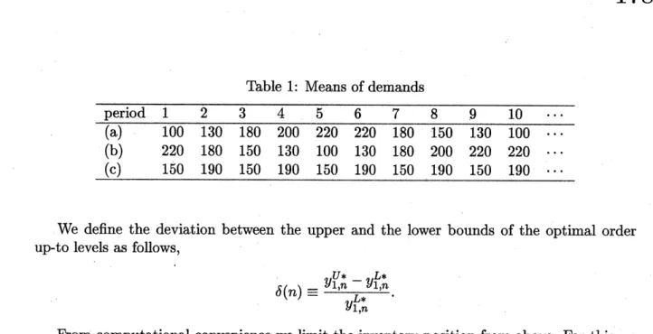
demand pattern: (a) increasing-decreasing, (b) decreasing-increasing and (c) almost stable.

Let the distributions of the demands be the normal distributions which are truncated to

become non-negative. The

means

of the demands for the three types ofdemandpattern

are

shown in Table 1. Let the standard deviation of the demand at each period be half of the

mean of the demand. Let the distributions of the production capacity be also the normal

distributions, and their standard deviation be 10. We change the

mean

of the production

capacity amongseveral values.

Let each parameter of the model like

below:

$c_{t}=\underline{\mathrm{c}}=\overline{c}=\mathrm{p}\mathrm{r}\mathrm{o}\mathrm{d}\mathrm{u}\mathrm{c}\mathrm{t}\mathrm{i}_{0\mathrm{n}}$cost $=30,$ $h_{t}=h=$

Table 1: Means of demands

$\overline{\frac{\mathrm{P}^{\mathrm{e}\mathrm{r}\mathrm{i}_{0}\mathrm{d}1234}5678910}{(\mathrm{a})100130180200220220180150130100}..\cdot..\cdot}$

(b) 220 180 150 130 100 130 180 200 220 220

.

.

.

(c) 150 190 150 190 150 190 150 190 150 190

.

.

.

We define the deviation between the upper and the lower bounds of the optimal order

up-to levels as follows,

$\delta(n)\equiv\frac{y_{1,n}^{U*}-y1,nL*}{y_{1,n}^{L*}}$

.

From computational convenience

we

limit the inventory position from above. For this we

assume

the following.

Assumption 1 The optimal order up-to levels$y_{t,n}^{*}$ are bounded, that is, there $exi\mathit{8}i\mathit{8}\overline{y}_{Su}ch$

that$y_{t,n}^{*}<\overline{y}$

for

all $n$ and$t<n$

.

We define

$\tilde{I}_{n+1,n}^{U}(_{X})=\{$

$0$ when $x>\overline{y}$,

$-\tilde{p}x/(1-\alpha)$ when $x\leq\overline{y}$

.

Then the following proposition holds.

Proposition 10 Under assumption 1 and using new $\tilde{I}_{n+1,n}^{U}(x)$

1. $y_{t,n}^{U*}\geq y_{t_{)}n}^{*}$

.

2. $y_{t,n}^{U*}\geq y_{t,n+1}^{U}*$.

Let $\overline{y}=300$ for the numerical examples. Table 2 shows the minimumplanning horizons

for which $\delta(n)$ is less than 0.05. From Table 2 we find that for the case that the demand

patternis increasing-decreasing and the production capacity constraint istight, the minimum

planning horizon gets longer than

ones

for other

cases.

This

means

that for the

increasing-decreasing demand

case we

have to consider the demands in much further future because of

the possibility that shortages may occur. On the otherhand, when the production capacity

constraint is not tight, the minimum planninghorizon for the increasing-decreasing demand

case

gets shorter. This is consistent with the results of $\mathrm{V}\mathrm{e}\mathrm{i}\mathrm{n}\mathrm{o}\mathrm{t}\mathrm{t}[?]$ for the inventory model

without the production capacity. The minimum planning horizons for the

cases

of the tight

production capacity constraint become longer than

ones

for other cases. This reflects the

effect that the sufficient production capacity contributes to reducing the influence of future

uncertainties ontheoptimal ordering policy.

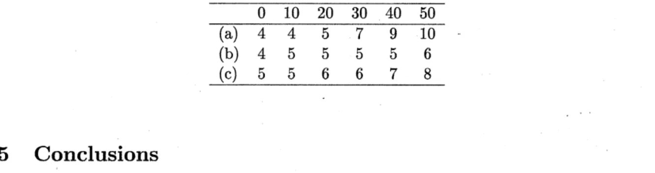
Next

we

investigate the effects of variance of the production capacity on the minimum

planning horizons. Table 3 shows the minimum planning horizons for several variances of

the production capacity. Let the

mean

of the production capacity be 220. From Table 3 we

find that as the variance of the production capacity becomes larger, the minimum planning

Table 2: Minimumplanninghorizons corresponding to several values ofmeanof production capacity

$\frac{200210220230240\cdots\infty}{(\mathrm{a})107433\cdots 2}$

(b) 5 5 5 4 4

...

3

(c) 8 6 5 4 4

...

3

makes the minimumplanning horizon much longer. However the effects of the variance of the

production capacity on the lengths of the minimum planning horizons are sufficiently small

when the variance is not large.

Table 3: Minimumplanning horizons corresponding to several values of standard deviation of production

capacity

$\frac{01020304050}{(\mathrm{a})4457910}$

(b) 4 5 5 5 5 6

(c) 5 5 6 6 7 8

5

Conclusions

In this paper

we

developed

an

equivalent formulation of the original production-inventory

problemwithuncertainproductioncapacity and uncertain demand. From the$\mathrm{f}o$rmulation the

upperand the lowerbounds ofthe optimal order up-to levelswerederived. Thenitwasshown

that the upper and the lower bounds of theoptimal order up-to levels converge respectively,

and under mild conditions the differences between the upper and the lower bounds converge

exponentiallyto zero.

Extensions to convex holding and penalty costs with bounded derivatives and fixed

lead-time are possible. Since the results in this paper depend on the convexity of cost functions

and the boundedness of their derivatives, the model can be extended to

convex

holding and

penalty costs with bounded derivatives. Also since the equivalent formulation developed in

this paper

uses

the inventory position as state, fixed leadtime can be incorporated into the model along the standard way.

References

[1] Bean,J. Smith,R. and Lasserre,J., ”Denumerablestate nonhomogeneous Markov decision

processes”, Journal ofMathematical Analysis and Application 153 (1990) 64-77.

[2] Bes,C. and Sethi,S.,”_{Concepts of forecast and decision horizons: applicationsto dynamic}

stochastic optimization problems”, Mathematics of Operations Research 13 No.2 (1984)

295-310.

[3] Ciarallo,F.W., Akella,R. and Morton,T.E., ”A periodic review, production planning

model with uncertain capacity and uncertain demand–optimality of extended myopic

[4] Federgruen,A. and Zipkin,P., ”An inventory model with limited production capacity and

uncertain demands I. The average-cost criterion”, Mathematics of Operations Research

11 No.2 (1986) 193-207.

[5] Federgruen,A. and Zipkin,P., ”An inventory model with limitedproduction capacity and

uncertain demands II. The discounted-cost criterion”, Mathematics of Operations

Re-search 11 No.2 (1986) 208-215.

[6] Glasserman,P. and Tayur,S., ”Sensitivity analysis for base-stock levels in multi-echelon

production-inventory systems”, Management Science41 No.2 (1995) 263-281.

[7] Glasserman,P. and Tayur,S., ”A simple approximation for multi-stage capacitated

production-inventory system”, Naval Research Logistics43 No.l (1996) 41-58.

[8] G\"ull\"u,R., ”Base stock policies for$\mathrm{p}\mathrm{r}\mathrm{o}\mathrm{d}\mathrm{u}\mathrm{C}\mathrm{t}\mathrm{i}_{0}\mathrm{n}/\mathrm{i}\mathrm{n}\mathrm{v}\mathrm{e}\mathrm{n}\mathrm{t}\mathrm{o}\mathrm{r}\mathrm{y}$ problems withuncertain capacity

levels”, European Journal of Operational Research 105 (1998) 43-51.

[9] Iida,T., ”The infinite horizon non-stationary stochastic inventory problem:

near

myopic

policies and weak ergodicity”, European Journal of Operational Research 116 (1999)

405-422.

[10] Iida,T., ”The Nonstationary Infinite Horizon Production-inventory Problem with

Un-certain Capacity and Uncertain Demand”, Technical Report, Department of Industrial

Engineering and Management, TokyoInstitute of Technology (1999).

[11] Karlin,S., ”Dynamic inventory policy with varying stochastic demands”, Management

Science 6 No.3 (1960) 231-258.

[12] Karlin,S., ”Optimal policy for dynamic inventory process with stochastic demands

sub-ject to seasonal variations”, JournalofSIAM8 No.4 (1960) 611-629.

[13] Kapu\’{s}citski,R. and Tayur,S., ”A capacitated production-inventory model with periodic

demand”, Operations Research 46 No.6 (1998) 899-911.

[14] $\mathrm{M}\mathrm{o}\mathrm{r}\mathrm{t}0\mathrm{n}:^{\mathrm{T}.\mathrm{E}}.$, ”The nonstationary infinite horizon inventoryproblem”, Management

Sci-ence

24No.14 (1978) 1474-1482.

[15] Morton,T.E. and Pentico,D.W., ”The finite horizon nonstationary stochastic inventory

problem: near-myopic bounds, heuristics, testing”, Management Science 41 No.2 (1995)

334-343.

[16] Veinott,A.F.,Jr., ”Optimal stockage policies with non-stationary stochastic demands”,

in: H.Scarf,D.GilfordandM.Shelly (eds.), Multistage InventoryModelsand Techniques,

Stanford University Press, Stanford, CA, 1963.

[17] Wang,Y. and Gerchak,Y., ”Periodic review production models with variable capacity,

random yield, and uncertain demand”, Management Science 42 No.l (1996) 130-137.

[18] Yano,C.A. and Lee,H.L.,”Lotsizing with random yields: areview”, Operations Research

43 No.2 (1995) 311-334.

[19] Zipkin,P., ”Critical number policies for inventory models with periodic data”