Interest Rate Policy: A Critical
Reconsideration Using a Dynamic Model
権利
Copyrights 日本貿易振興機構(ジェトロ)アジア
経済研究所 / Institute of Developing
Economies, Japan External Trade Organization
(IDE-JETRO) http://www.ide.go.jp
シリーズタイトル(英
)
Occasional Papers Series
シリーズ番号
39
journal or
publication title
Overcoming Asia's Currency and Financial
Crises: A Theoretical Investigation
page range
22-40
year
2004
2
The Asian Currency Crisis and
IMF High Interest Rate Policy:
A Critical Reconsideration
Using a Dynamic Model
I.
Introduction
There has been a great deal of criticism voiced against the International Monetary Fund’s prescription for dealing with the Asian currency crisis. Radelet and Sachs (1998) argued that the closure of banks in Indonesia in November 1997 brought on investor panic which worsened the crisis. Feldstein (1998) argued that the incorporating of structural reform policies with conditionality was inappropriate for dealing with the short-term liquidity crisis. Rodrick (1998) and Bhagwati (1998) called into question the IMF’s intention of liber-alizing capital transactions. Bhagwati also criticized the powerful influence on the IMF of the close relationship between the U.S. Treasury Department and Wall Street financial institutions through their exchange of personnel, what Bhagwati calls “a Wall Street-Treasury complex,” which has had a significant influence on the formulation of IMF policies. Even the World Bank (1998), the IMF’s “Bretton Woods sister institution,” has discreetly criticized the failure of IMF policies to cope with the Asian crisis. Noteworthy in this criticism has been the reference to monetary policies, attesting to doubts among many about the effectiveness of IMF intentions to maintain stable exchange rates through high interest rate policies.
The IMF (1999) itself came to acknowledge some of these criticisms. It admitted that at the start of the Asian currency crisis it miscalculated the severity of the crisis, and that its excessively tight fiscal policy had been
inappropriate. However, it did not waver in its attitude that high interest rates were needed to stabilize exchange rates, and it maintained this attitude even in the face of the Brazilian currency crisis at the start of 1999 when international investors were expecting a cut in interest rates; the IMF instead insisted that Brazil raise interest rates.
Joseph Stiglitz (2002), formerly of the World Bank, sharply criticized the way the IMF dealt with the Asian currency crisis, saying in part that following the crisis it should have stimulated the affected economies. In reaction to this criticism, the IMF made a frank admission there had been mistakes in its policy in the aftermath of the crisis, with the exception of its high interest rate policy. Thus despite such admission, and the need for “honest debate and a closer look at the evidence” (Dawson 2002), the IMF’s basic stance of “restor-ing external confidence by rais“restor-ing interest rates” (ibid.) continues unchanged. Thus the correctness of high interest rate policy remains an important issue in the debate surrounding the IMF’s prescription for curing the Asian currency crisis. Kashiwabara and Kunimine (1999) examined the issue and came to four conclusions: (1) high interest rates worsened the crisis in domestic financial systems, (2) stimulating capital inflow through high interest rates increases the probability of future instability in capital flows, (3) high interest rates are inappropriate as an anti-inflation measure, and (4) alternatives to high interest rate policies should be considered.
All the above criticisms point out the serious side effects of high interest rate policies. But none look into whether or not these policies are effective in maintaining exchange rates, which of course is the original intent of such policies. This study seeks to clarify this issue. In so doing, it will undertake a theoretical examination using a dynamic model of exchange rates. There is a problem however. The IMF has not clearly defined what sort of model its own theoretical model is. This seems to be due to the fact that the IMF has always been too confident of its high interest rate policy.
Up to now the IMF has been satisfied with the simple explanation that “high interest rates restore investor confidence in the currency.” Therefore it has not shown much interest in presenting a more deeply penetrating theoretical model. Recently it has provided a roughly sketched model in IMF (1999). The model is still too simple and insufficiently explanatory, but it is set forth in equations and therefore there is no possibility of it being misinterpreted. Hereafter in this study this model will be referred to as the IMF model, and it will be explained in Section II. The particular feature of this model is its employment of an exogenous variable known as “risk premium.” The problems with this variable will also be discussed in Section II. The IMF model, unfortunately, is extremely deficient in its examination of short-term macroeconomic
stabiliza-tion policy. However, by introducing a few addistabiliza-tional short-term dynamic propositions, the IMF model can be expanded into a dynamic model that looks much like Dornbusch’s “overshoot model” of exchange rates (Dornbusch [1976]). This point is taken up in Section III. Further still, by changing the premises of this dynamic model only slightly, it can be shown that high interest rate policies cannot be justified. The issue here is whether or not the long-term equilibrium level of real exchange rates changes. If for example the long-term equilibrium level is shifting toward real depreciation and a high interest rate policy as advocated by the IMF is carried out, an unnecessary deflationary adjustment process will occur, an issue taken up in Section IV. In Section V, we use Thai economic data to examine the possibility that this sort of defla-tionary adjustment actually did take place. Finally in Section VI, we will examine the possibility that risk premium is determined endogenously in response to policies and is not an exogenous variable. This would mean that high interest rate policy itself could become the cause for the occurrence of risk premium.
II.
The IMF Model
In IMF (1999) the following model is presented:
mt− pt=αyt−βit, (2.1)
it= i*+ et
+1− et+πt, (2.2)
pt= p*+ et− qt. (2.3)
All of the variables except nominal interest rate are logarithms; m, p, y, i, e, π, and q indicate, respectively, money supply, price level, real GDP, nominal interest rates, nominal exchange rates, risk premium, and real exchange rates. Variables with “*” indicate corresponding variables in foreign countries. α and β are constants indicating, respectively, income elasticity and interest elasticity of money demand.
One notation in this study differs from that used in IMF (1999); this is “q” the symbol for real exchange rates. In IMF (1999) µ is used while its equiva-lent in this study is “−q.” Therefore the reader needs to be aware that an increase and decrease in this variable in this study means the reverse of that in IMF (1999). In other words, in the model used in this study, a rise in the numeric value of q means a depreciation in real exchange rates. The advan-tage of this modification is that it is consistent with the symbol of the variable for nominal exchange rates. For nominal exchange rates too, in this study a rise in the numeric value of variable e means a depreciation in nominal exchange rates.
Briefly explaining each part of the IMF model, equation (2.1) expresses money market equilibrium; equation (2.2) expresses the relationship of inter-est parity with risk premium; equation (2.3) is the definition of real exchange rates. Each of these is a basic equation of international macroeconomics. A model combining these equations is regarded as simply describing long-term equilibrium in a small open economy. Here short-term price stickiness is not assumed, therefore it must be born in mind that this model is intended for analyzing the long-term equilibrium.
Though not stated clearly in IMF (1999), the variables p, i, and e in the model are regarded as endogenous variables. The model can be solved as a difference equation of e giving the following result:1
e(t) = (mt+j− αyt+j+ βπt+j+ qt+j). (2.4)
However, for the sake of simplification, the exogenous variables i* and p* have been regarded as zero.
In this model, m, y, π, and q are exogenous variables (m in particular being a policy variable). When it is assumed, for the sake of simplicity, that these do not change over time, equation (2.4) becomes
e(t)= m − αy + βπ + q. (2.5)
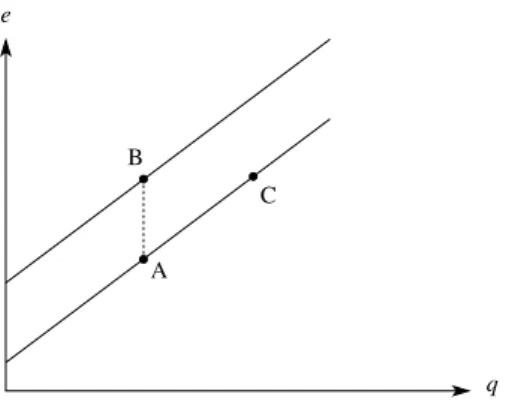
Focusing on the relationship between e and q, when equation (2.5) is drawn on the q–e plane, it forms a upward sloping straight line like that in Figure 2-1. Either expansion of the money supply or rise in risk premium causes an upward shift of this straight line. This shift means that e rises (i.e., nominal
e
q B
A
C
Fig. 2-1. The Relationship between Nominal and Real Exchange Rates in the IMF Model
1 1+β β 1+β
j ∑∞ j=0exchange rates depreciate) with q being unchanged, i.e., a movement such as that from point A to point B takes place. Reducing m (i.e., a tight monetary policy) can work to prevent this depreciation in nominal exchange rates; and such a policy is desirable to cancel out the original shift (i.e., to shift the straight line back downward to its original level).
One of the features of the IMF model is its inclusion of the exogenous risk-premium variable. Without this variable it becomes a model for observing the relationship between money supply and exchange rates in long-term equilib-rium, where an expansion in the money supply will not have an effect on other real variables (particularly real exchange rates); in short it will exhibit an open economy’s version of “long-run monetary neutrality” with only the domestic price level and nominal exchange rate having the same magnitude of change. Qualitatively the risk premium term performs the same function as the money supply term, i.e., it causes nominal exchange rate depreciation (and a rise in the price of goods). Thus the policy implication is that a tight monetary policy (i.e., high interest rate policy) is needed to counteract the effects of a rise in risk premium.
But this is a totally inadequate argument because, as already noted, this model analyzes long-term equilibrium, while coping with the currency crisis is a problem of short-term stabilization. Therefore focusing only on changes in long-term equilibrium can lead to mistaken policies. Short-term dynamics also should be examined.
Moreover, it is unusual in a long-term model to put importance on risk premium. That risk premium will continue rising over the long term can hardly be called an adequate assumption. It has to be explained whether (i) risk premium is assumed to rise only over a given short-term period, or (ii) special reasons exist for risk premium to continue rising over the long term. In the first case, the temporary short-term rise will have only a very small effect on long-term equilibrium, in which case risk premium could largely be ig-nored as a factor affecting long-term equilibrium. If the IMF model is applied carefully, π in the Σ sign on the right side of equation (2.4) will have a positive value only at a certain specific point of time, and therefore the effect on e should be very small. In the second case where risk premium continues over the long term, such a situation would probably be better understood as some sort of fundamental change in the structure of the economy rather than being regarded as risk premium. Whatever the case, there is no persuasive explana-tion anywhere in IMF (1999) of this issue. So why has the IMF felt compelled to put risk premium at the center of its model? Because prior to the currency crisis in East Asia, it was not at all pursuing an loose monetary policy like the monetization of fiscal deficit; and now it finds itself with no way of explaining
the need for its high interest rate policy other than introducing the risk pre-mium variable.
In addition to the above, there has been insufficient examination of other exogenous variables in the model. A particular problem is the lack of inquiry into changes in q, the real exchange rate. Given the conditions of the currency crisis, it is highly possible that there will be changes not simply in nominal exchange rate but also in the desirable level of real exchange rate. It has even been argued that one of the factors for the currency crisis was the concern that real exchange rates were overvalued. Regarding the possibility of change in the level of desirable exchange rate (hereafter termed “long-term equilibrium real exchange rate”), there is for example the situation where a country’s expected future burden of debt servicing suddenly expands. In such a situation there has to be additional improvement in the country’s current account bal-ance just to cover the increased debt servicing. Usually this is achieved through a rise in q (i.e., depreciation of the real exchange rate).2 This does not mean there is a sudden movement from point A to point B in Figure 2-1, even though during the currency crisis a rise in nominal exchange rate was ob-served. Rather it would be more appropriate to understand it as a movement from point A to point C in Figure 2-1. In this situation the factor bringing about a depreciation in nominal exchange rate is not the rise in risk premium but the depreciation in long-term equilibrium real exchange rate. To carry out a tight monetary policy in this situation is to introduce disturbances that will retard adjustments in the economy.
III.
Extension of the IMF Model and Short-Term Exchange Rate
Dynamics
This section will look at the failure of the IMF model to take into consider-ation short-term dynamics. In order to do this, we would first like to present a dynamic model with a number of added premises (equations) which expand the IMF model.3
It will be seen that this model largely coincides with Dornbusch’s overshoot model which is the standard model for the dynamic analysis of international macroeconomics. It describes the dynamic transition process from a Keynesian short-term economic world where prices are sticky to a long-term equilibrium where prices are flexible. The basic equations of the IMF model, equations (2.1)–(2.3), can be utilized just as they are. Two equations will be added, one describing the possibility of a discrepancy from full-employment GDP over the short term (a Keynesian proposition) and another describing a gradual
price-level adjustment in accordance with the modified Phillips curve (equa-tions (2.A.1) and (2.A.2) in the Appendix 2-1). In this way the basic equa(equa-tions of the IMF model are maintained so that the steady state of this dynamic model coincides with equilibrium in the IMF model (i.e., the economy’s long-term equilibrium). (A detailed description of this expanded model is shown in the Appendix 2-1.)
The essential points of this model are diagrammed in Figure 2-2a. As with the figures in Section II, the vertical axis is nominal exchange rate (e) and the horizontal axis is real exchange rate (q) (both are logarithms). Also as in Section II, for both e and q, a rise in their numeric values means depreciation. It is assumed that over a momentary period of time prices are sticky. Therefore a change in the nominal and real exchange rates should be perfectly correlated at any given moment of time, which means that at any given moment of time e and q must move along the 45-degree line of the graph.
Here $q is taken as the level of long-term equilibrium real exchange rate. The perpendicular dotted line is the q = $q line, and long-term equilibrium has to be on this line. Curve SS describes the trajectory path that the economy will trace when it diverges from long-term equilibrium under the assumption of rational expectations. This curve will shift upward with either an increase in the money supply or risk premium.
We start from point A where the economy is at long-term equilibrium or, using a term of dynamic analysis, in a steady state. We use the words “long-term equilibrium” and “steady state” interchangeably. Now let us suppose that curve SS shifts upward to S′S′ due to a permanent increase in the money supply (or risk premium). As stated earlier, nominal and real exchange rates
Fig. 2-2
a. Overshoot b. Changes in the Endogenous Variables over Time
e q t B A C S′ S S′ S q¯ (When π rises) (When m rises) π p e, q, y i
can move only along the 45-degree line at any given instant. Therefore at the instant the shift of SS occurs, the economy immediately moves to point B (both nominal and real exchange rates depreciate). The economy will now be aligned with trajectory S′S′ where it will gradually adjust until it is at point C. On this trajectory both nominal and real exchange rates gradually appreciate. But when the economy at C is compared with its original equilibrium at A, real exchange rate is still the same and only nominal exchange rate has depreciated, meaning that price levels have increased. Thus the dynamic process from B to C must coincide with the gradual rise of domestic prices.
This momentary depreciation of nominal exchange rate and then its gradual appreciation is called “overshoot.” This dynamic process causes real GDP to exceed full employment levels, which brings on a price rise in accordance with the modified Phillips curve. Also with the dynamic process from B to C, the level of nominal interest rate is below that of long-term equilibrium. The amount of decrease in interest rate will be equal to the expected rate of appreciation in nominal exchange rate involved in the dynamic process in accordance with interest rate parity in equation (2.2). However, when the shift of curve SS occurs because of an increase in risk premium and not because of an increase in money supply, it is possible that interest rate will be higher than its equilibrium value even with the dynamic process (when the increase in risk premium exceeds the expected rate of appreciation in exchange rate). Figure 2-2b describes the changes in the endogenous variables over time. A major difference from the model presented in the previous section is that in the model in this section both q and y are endogenous variables; and the changes that occur in these two are the same kind as that in e.
If the shifting of the risk premium (which is an exogenous variable) is excluded, the above model is exactly like Dornbusche’s overshoot model. The important point here is that the effect caused by an increase in risk premium is qualitatively the same as the effect caused by an increase in money supply. Thus if an increase in risk premium leads to a currency crisis, then a tight monetary policy is a desirable counter measure; the money supply is reduced, and the S′S′ curve is shifted back down to SS. This will maintain the economy’s steady state at point A.
Up to this point the policy implication is the same as in the IMF model. But we undertook this careful examination of the short-term dynamic process because it will be needed to better clarify the danger in the IMF’s logic, which will be taken up in the next section.
IV.
Change in Equilibrium Exchange Rate and the Possibility of
Excessively Tight Monetary Policy
Even with the short-term dynamic model presented in Section III, it is impor-tant to consider the possibility of change taking place in $q, the long-term equilibrium real exchange rate (indicated by q in the model in Section II). Leaving all other conditions unchanged, let us examine the case where $q is assumed to change to $q′ (assuming $q < $q′). This is shown in Figure 2-3a, and in this case, too, curve SS shifts upward. However, after this shift to S′S′, it will come to intersect perpendicular line q= $q′ at point B. Therefore the momen-tary movement of economy from its original point A to point B is the same as in the previous model, but B in this model becomes a new long-term equilib-rium, and no further dynamic adjustment process is needed.4
Thus the correct policy toward a shift in nominal exchange rates due to a change in $q is to let the shift take place. In effect, “leaving it to the market” becomes the best approach, and a tight monetary policy is unnecessary. The point is that if an adjustment in the real exchange rate is necessary, the IMF’s high interest rate policy is misguided.
Supposing that in the above situation a misguided high interest rate policy were carried out. What would happen? Let us say that although $q was really rising, observers of the situation did no believe it was rising. To these observ-ers the situation was not like that of Figure 2-3a; rather they perceived it as in Figure 2-2a. In effect they saw the change from A to B not as one of a change from one point of long-term equilibrium to another point of long-term
equilib-Fig. 2-3
a. A Change in Equilibrium b. Changes in the Endogenous Real Exchange Rates Variables over Time
e q t B A S′ S S′ S q¯ q¯′ e, q i, p, y
rium, but as a short-term overshooting. But the observers would find it strange that the money supply was not increasing, and therefore they could come to the conclusion that this change was due to a rise in risk premium.
As a result of such observations, it could be decided that a tight monetary policy would be suitable to counter the situation. Figure 2-4a shows the effects of such a mistaken tight monetary policy. The implementation of the policy prevents curve SS from shifting to S′S′, therefore the latter is shown as a dotted line. Instead, point C, where curve SS and q= $q intersect, becomes a new steady state. However, over a momentary period of time, the economy can only move along the 45-degree line, thus it cannot help but remain at point A.5 Then it will gradually move in a dynamic trajectory along curve SS toward C. In other words, the mistaken tight monetary policy will lead to an unneeded adjustment process.
There is no overshooting in nominal or real exchange rates. Instead both e and q slowly continue to depreciate toward point C. Equilibrium of the money market under rational expectations makes high interest rates necessary to offset the continuing depreciation. Thus this adjustment process becomes a dismal deflationary adjustment trajectory of sustained exchange rate depre-ciation with prolonged high interest rates. Looking at the changes in the endogenous variables over time, diagrammed in Figure 2-4b, the change in y is of particular interest. Initially y suffers a big fall from its full employment level, then slowly rises back toward its original level. This is very different from the case of an overshoot discussed in the previous section (see Figure 2-2b) where directly after devaluation, y exceeded the level of full employment. Compared with this latter, the situation described in Figure 2-4b conforms a
Fig. 2-4
a. Mistaken Tight Monetary Policy b. Changes in the Endogenous Variables over Time
e q t B A C S′ S S′ S q¯ q¯′ p y e, q i
great deal more with the real events that occurred in East Asia.
In the next section we would like to take a closer look at this conformity with East Asian events in another way, focusing in particular on the move-ments that took place in Thai exchange and interest rates. However, our aim here is not a precisely gauged proof of the effects of high interest policy; rather we want to use the example of Thailand in order to test the effects of alternative policies as analyzed in the models presented in this study.
V.
Thailand as an Example
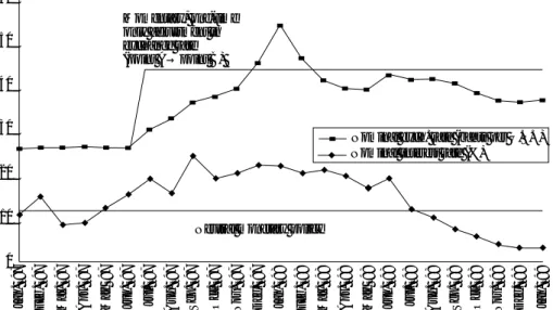
The movements that took place in Thai nominal exchange rate and short-term interest rate are shown in Figure 2-5. It can be seen that changes in the exchange rate that began in mid-1997 had largely settled down by the end of 1998 and the beginning of 1999. During this latter time frame the economy can be regarded as attaining a new long-term equilibrium, or steady state. A comparison of mid-1997 with the latter time frame shows that the nominal exchange rate had risen (depreciated). During this period the degree of price rise was less than that of the depreciation in the nominal exchange rate, meaning that the real exchange rate also depreciated. This is in agreement with the assumption presented in the previous section that long-term
equilib-Nominal exch. rate (bahts per U.S.$) Partially
overshoot Original steady
state (point A)
Extremely long period of tight money policy (about one year)
New steady state (point C)
Jan. ’97 Feb. ’97 Mar. ’97 Apr. ’97 May ’97 Jun. ’97 Jul. ’97 Aug. ’97 Sep. ’97 Oct. ’97 Nov. ’97 Dec. ’97 Jan. ’98 Feb. ’98 Mar. ’98 Apr. ’98 May ’98 Jun. ’98 Jul. ’98 Aug. ’98 Sep. ’98 Oct. ’98 Nov. ’98 Dec. ’98 Jan. ’99
60 50 40 30 20 10 0
Nominal interest rate (%)
Fig. 2-5. Movement of Thai Nominal Exchange Rates and Short-Term Interest Rates, 1997–99
rium real exchange rate will depreciate ($q→ $q′). To put it differently, we can regard the situation during the first half of 1997 as corresponding to point A in Figure 2-4a (original steady state) and the situation after the end of 1998 as corresponding to point C (new steady state).
The level of interest rate on the call market indicated the nature of monetary policy during this time period. For a little over a year the over-night interest rate was kept around 20 per cent, showing that a constantly tight monetary policy was in effect. From mid-1997 until the end of that year the nominal exchange rate depreciated in a sustained series of movements which also accords with the movement diagrammed in the model in the previous section. In effect, Thailand experienced a dynamic process brought on by a high interest rate policy that hampered the adjustment needed in exchange rate.
However, the movement of the exchange rate during the period from the end of 1997 to the beginning of 1998 is inconsistent with the model in the previous section. The movement during this period can be suitably explained as an exogenous rise in risk premium. The constant level of interest rate shows that there was no further tightening of monetary policy. During this time, however, the nominal exchange rate experienced a sudden rapid depreciation, then a quick re-appreciation back to its immediately previous level. These events spanned a period of about three months.
This period coincided with a time of political instability and a rapid depre-ciation of exchange rates in Indonesia and the Republic of Korea, which greatly worsened the view of international financial markets toward the East Asian economies as a whole. Thus it could be said that this movement was indeed due to a rise in risk premium. It is important to note that this sort of rise in risk premium is over the short term. In the Thai example it was two to three months at the most. With the end of risk premium rise there was also a quick end to the overshoot of the nominal exchange rate.
Let us suppose for the sake of conjecture that Thailand had not followed a high interest rate policy. What sort of movement in the exchange rate would have taken place? It will be assumed here that no rise at all took place in risk premium and that the sudden increase (depreciation) in the long-term equilib-rium real exchange rate was the cause for the currency crisis. With monetary policy kept neutral, there would be no short-term dynamic process, and the economy would immediately move to a new long-term equilibrium. There-fore, the interest rate is drawn as a horizontal straight line, and the nominal exchange rate is drawn showing a momentary, one-time only adjustment taking place. This is shown in Figure 2-6 where straight lines are drawn over the movements of the actual exchange and interest rates. The jump in the nominal exchange rate corresponds to the shift from A to B in Figure 2-3a.
The level of the nominal exchange rate after adjustment is higher than the actual exchange rate, but this corresponds to the horizontal distance between C and B in Figure 2-4a. The difference is that when there is a momentary shift to B, there is no deflationary process that comes with a high interest rate policy; therefore the real exchange rate ($q′) will settle at C with the nominal exchange rate being higher (more depreciated).
What would happen if the rise in risk premium from the end of 1997 to the beginning of 1998 were introduced into our conjecture? As was already stated, during this period overshoot did actually occur. Therefore ideally a high interest rate policy should have been applied only during this period, and with the decline in risk premium, there should have been an immediate return to a neutral monetary policy. This is a sort of “fine-tuning” of the economy.
Is such a fine-tuning policy realistic? This can be thought of as an analogy of the argument between Keynesians and monetarists over discretionary policy. Monetarists argue that when the government cannot recognize the state of business conditions in a proper and timely manner, discretionary macroeco-nomic policy cannot stabilize the economy; it will only destabilize it. In the same way, when changes in risk premium are not recognized in a proper and timely manner, the government can misread the need for a high interest rate policy.
Looking at the Thai data once again, there is no indication that interest rate
60 50 40 30 20 10 0
Jan. ’97 Feb. ’97 Mar. ’97 Apr. ’97 May ’97 Jun. ’97 Jul. ’97 Aug. ’97 Sep. ’97 Oct. ’97 Nov. ’97 Dec. ’97 Jan. ’98 Feb. ’98 Mar. ’98 Apr. ’98 May ’98 Jun. ’98 Jul. ’98 Aug. ’98 Sep. ’98 Oct. ’98 Nov. ’98 Dec. ’98 Jan. ’99
Nominal exch. rate (bahts per U.S.$) Nominal interest rate (%)
Momentary, one-time only adjustment in exchange rate (point A→point B)
Neutral monetary policy
Fig. 2-6. Conjectured Movement in the Thai Exchange Rate (Had a High Interest Rate Policy Not Been Taken)
moved appreciably during the late 1997 early 1998 time period although it was clearly thought that exchange rate depreciated because of a rise in risk premium. In effect, further monetary tightening did not take place. This sug-gests that the Thai government and/or the IMF failed to recognize a rise in risk premium in a timely manner.
How about “proper recognition,” the other condition needed for a success-ful discretionary policy? In theoretical models risk premium is just one of the exogenous variables used. Thus it is a delusion to think it an easy task to properly recognize risk premium. A good analogy here is with the exogenous variable “A” or “technological progress” in the Solow growth model. A body of research based on endogenous growth theory now explains technological progress as an endogenous variable. As a result, it is now considered that the exogenous variable of technological progress in the Solow model should be explained endogenously by multiple factors such as the effects of human capital accumulation and learning-by-doing, or the expansion of knowledge through R&D. This is not simply a theoretical problem; it has an effect on policy implications as well. For example, if technological progress is achieved through human capital, then it becomes important to invest in education. If, on the other hand, such progress can be better attained through R&D, then the government’s technological policies become important. In the same way, if risk premium were also to be explained by a multiple of factors, the differ-ences in the explanatory factors would be expected to have an effect on policy implications.
The next section will examine this point using the model framework in Section IV. It will point out the possibility of risk premium occurring endog-enously through the interaction with policy. The purpose of doing this is to show a counter example against the appropriateness for treating risk premium as an exogenous variable, and we do not insist that risk premium is solely caused by misguided policy. However, we think that it is enough to indicate the danger in the “one-size-fits-all” formula of using high interest rates to counter currency crises whenever and wherever they break out.
VI.
Endogenous Risk Premium
This section also looks at a situation where a tight monetary policy has been mistakenly implemented due to misconceptions about the economy. As pointed out earlier, in such a situation, the economy enters into an unnecessary defla-tionary adjustment process. During that process long-term equilibrium q (i.e., $q) and the actual q differ. The significant characteristic of this adjustment
process is that it is possible at any point in time to immediately achieve long-term equilibrium through a policy change. The only thing needed is to have nominal and real exchange rates depreciate at once. As shown in Figure 2-7a, during the adjustment process from A to C, the economy can move to long-term equilibrium through a momentary exchange rate adjustment (deprecia-tion) along the 45-degree line (the move to point D in the figure). At this time discrete exchange rate depreciation takes place.
Rational private economic agents would take into account the risks from this sudden policy change and would act accordingly. The momentary ex-change rate depreciation induced by the policy ex-change would cause capital losses, so investors would likely call for higher interest rates, but only high enough to cover the possibility of their losses. When λ represents the prob-ability of policy change, the interest parity equation6 becomes
i= i*+ e(t + 1) − e(t) +λ[$q′ − q(t)].
When equation (2.2) is compared with this equation, risk premium π in equa-tion (2.2) can be regarded as
π = λ[$q′ − q(t)]
and can be explained endogenously. In other words, it is the mistaken policy itself that produces the risk premium. By misreading the situation, a high
e q t B A C D S′ S S′ S q¯ q¯′ p y e, q i Fig. 2-7
a. The Possibility of a Sudden Policy b. Changes in the Endogenous Change during the Adjustment Process Variables over Time
Note: The dotted lines indicate the trajec-tory of change in the endogenous variables over time when a sudden policy change occurs during the adjustment process.
interest rate policy may in an ironically self-fulfilling way make a high inter-est rate necessary. Of course such a situation would immediately bring a halt to the high interest rate policy permitting a reduction in nominal and real exchanges rates which could eliminate the risk premium. Thus high interest rate policy is a misreading and therefore an inappropriate policy.
A cautionary note is needed here. The present discussion is to point out the possibility that a part of risk premium is caused by uncertainty over policy implementation; it is not arguing that all of risk premium is due to such uncertainty. But because risk factors other than policy implementation uncer-tainty are not taken into consideration here, in this discussion, risk premium π is explained totally by this uncertainty. This is solely for the sake of simplicity. If other factors of uncertainty were introduced, π could be decomposed into a multiple of factors.
VII.
Conclusion
This study looked at the IMF’s high interest rate policy as it pertains to the Asian currency crisis. It expanded the IMF’s model into a dynamic model through which it examined the relationship between interest rate policy and exchange rate in the short run. It then pointed out the possibility of a high interest rate policy inducing an unnecessary deflationary adjustment process, and sought to verify this point using Thai data. This study also examined the possibility that the high interest rate policy itself could lead to uncertainty which would cause risk premium to rise endogenously. The following four points encapsulate the main arguments of this study.
1. The IMF’s theoretical model is suitable for analyzing long-term equi-librium. By incorporating several additional propositions into this model, it is possible to construct a short-term dynamic model, which is a sort of Dornbusch overshoot type. Those models in themselves are appropriate from the theoreti-cal viewpoint.
2. But how to use those models to get policy implications is another matter. It seems that the IMF had no qualms about its conclusion (i.e., the need for high interest rate policy). Two points in particular that need careful consideration are the way of handling risk premium as an exogenous variable and the possibility of change in the level of long-term equilibrium real ex-change rate.
3. Thailand’s experience as shown from the Thai data strongly suggests that its IMF-type high interest rate policy simply hampered the process of inevitable change, i.e., depreciation of the real exchange rate.
4. It is possible that the IMF’s high interest rate policy itself was one cause for the rise in risk premium.7
All of the models used in this study are based on fundamental textbook models of international macroeconomics. But even with these fundamental models, it was shown that a slight difference in assumptions will bring about a great difference in policy implications. In future studies analysis using dy-namic models needs to be further refined, and data for other countries (Indo-nesia, Korea, and Malaysia) that experienced the currency crisis need to be examined.
Appendix 2-1
Here two assumptions are added to equations (2.1)–(2.3). One is that the discrepancy between long-term equilibrium real exchange rate ($q) and the actual rate (q) causes a discrepancy between full employment GDP and actual GDP. The other is that the price level (p) cannot be adjusted in the short run, but that it will gradually change in response to excess supply (by falling) or excess demand (by rising) in accordance with the modified Phillips curve. The equations for these two assumptions are shown below (with all of the vari-ables except nominal interest rate being logarithms).
yd= $y +δ(q − $q), (2.A.1)
p(t+ 1) − p(t) =φ(yd
t− $y) + ~p(t + 1) − ~p(t), (2.A.2) where ~p(t) is the price level at full employment GDP and ~p(t)≡ e(t) + p*− $q; yd, $y, and $q are actual GDP, full employment GDP, and long-term equilibrium real exchange rate, respectively; δ and φ are positive constants; and t is the time parameter.
Because
~p(t)− p(t) = e(t) + p*− p(t) − $q = q(t) − $q
then, from equation (2.A.2) q(t+ 1) − q(t) = −φ(yd
t− $y).
When this is combined with equation (2.A.1), then q(t+ 1) − q(t) = −φδ (q(t) − $q),
and the solution to this difference equation is q(t+ j) − $q = (1 −φδ)j(q(t)− $q).
If 0 < 1−φδ < 1, which is assumed to be true, q will monotonously con-verge to its long-term equilibrium value $q.
When e(t) is calculated using the above, then
e(t)= (mt+j−α[$y + δ (qt+j− $q)] + βπt+j+ qt+j) = (mt+j−α$y + (1 − αδ)(qt+j− $q) +βπt+j+ $q)
= (mt+j−α$y + (1 − αδ)(1 − φδ)j(qt− $q) +βπt+j+ $q) = (mt+j+βπt+j)+ (qt− $q) −α$y + $q. To simplify further, when m, π are held constant, and $y = 0, then
e(t)= m +βπ + (qt− $q) + $q.
This equation is a more generalized version of equation (2.5) in Section II (with the inclusion of short-term dynamics). This can be confirmed by the fact that equation (2.5) will be obtained by substituting $q for qt in the above equation.
This equation describes curve SS in the figures in the previous sections. In this study the inclination of this curve is drawn as upward sloping, but a downward sloping curve can happen just as well. This will depend on the sign of 1−αδ. Usually it is assumed as upward sloping (Obstfeld and Rogoff [1996]). But whether SS is rising or falling has no effect on long-term equilib-rium. The difference comes in the short-term adjustment process where un-dershoot occurs instead of overshoot. Since this difference has no substantial effect on the main conclusions, an upward sloping curve has been assumed in this study (i.e., 1−αδ > 0).
1−αδ 1+βφδ 1−αδ 1+βφδ 1 1+β β 1+β
j ∑∞ j=0 1 1+β β 1+β
j ∑∞ j=0 1 1+β β 1+β
j ∑∞ j=0 1 1+β β 1+β
j ∑∞ j=0Notes
The present chapter has been revised based on Kunimune (1999a, 2000c).
1 The absolute value of β / (1 + β) is assumed to be less than one. Otherwise the value of equation (2.4) will not converge (causing divergence or oscillation). 2 When the international transfer of capital takes place, there is a question of
whether a change in real exchange rate is needed. This is called the “transfer problem” and is a classic issue in international economics. Other than in ex-tremely specific situations, the standard understanding is that a change is needed. See Dornbusch, Fischer, and Samuelson (1977).
3 Another very interesting short-term dynamic model for expanding the IMF model is the model known as “speculative attack.” This model tries to clarify the mecha-nism whereby a fixed exchange rate system is broken down by exchange rate speculation. However, fixed exchange rate systems in crisis-ridden countries have now largely been abandoned making this model irrelevant. The present study focuses on the effects of trying to stabilize exchange rate through high interest rate policy, therefore a floating exchange rate regime has been taken as a premise. There is another important model which includes government budget con-straints for cases like those in Central and South America where for a time governments relied on printing money which tied government fiscal conditions closely with monetary policy making it difficult to separate the two. For the East Asian countries, however, before the currency crisis hit, their fiscal conditions were very satisfactory; moreover none of the governments had ever resorted to the practice of printing money to generate revenues. Because of these great differ-ences, this kind of model’s extension was not adopted in this study.
4 To explain why this is so, it must be remembered that the steady state in this study’s model is equivalent to long-term equilibrium in the IMF model. Therefore equation (2.5) in Section II should be fulfilled in the steady state of this study’s model. If e and q in long-term equilibrium in equation (2.5) are graphed, they will fall along the 45-degree line. Meanwhile, as already stated in this study, e and q over a momentary period of time will move along the 45-degree line.
For these reasons, we can conclude that if A is a steady state, then B is also a steady state, and the move from A to B can occur instantaneously.
5 This explanation is inappropriate in a case where the inclination of curve SS happens to be 45 degrees. But this will not happen because as shown in the Appendix 2-1, the inclination of SS is 1−αδ, and since α, δ > 0, the inclination of
SS will be less than 45 degrees.
6 Here it is assumed that investors are risk neutral. If they are risk averse, they will demand higher risk premium, but this will not change the essence of the model. 7 However, there is also the opinion, as exemplified by Marchesi and Thomas
(1999), that “IMF lending programmes could be useful in resolving the debt crisis by acting as credible indicators for the country’s willingness to respond to debt relief by increasing investment and debt repayments.” (p. C124)