Negative Bubbles and Unpredictability of
Financial Markets: The Asian Currency Crisis
in 1997
著者
Kuchiki Akifumi
権利
Copyrights 日本貿易振興機構(ジェトロ)アジア
経済研究所 / Institute of Developing
Economies, Japan External Trade Organization
(IDE-JETRO) http://www.ide.go.jp
journal or
publication title
IDE Discussion Paper
volume
65
year
2006-06-01
INSTITUTE OF DEVELOPING ECONOMIES
Discussion Papers are preliminary materials circulated to stimulate discussions and critical comments
Abstract
We obtain the three following conclusions. First, business cycles depend on prices of stocks and primary commodities such as crude oil. Second, stock prices and oil prices generate psychological cycles with different periods. Third, there exist cases of “negative bubble” under certain conditions. Integrating the above results, we can find a role of a government in financial market in developing countries.
DISCUSSION PAPER No. 65
Negative Bubbles and
Unpredictability of Financial
Markets: The Asian Currency Crisis
in 1997
Akifumi KUCHIKI*
June 2006
Keywords: cycles, unpredictability, negative bubbles, governments JEL classification: G18, O16.
Executive Vice President, Japan External Trade Organization (JETRO) E-mail: [email protected]
The Institute of Developing Economies (IDE) is a semigovernmental, nonpartisan, nonprofit research institute, founded in 1958. The Institute merged with the Japan External Trade Organization (JETRO) on July 1, 1998.
The Institute conducts basic and comprehensive studies on economic and related affairs in all developing countries and regions, including Asia, Middle East, Africa, Latin America, Oceania, and East Europe.
The views expressed in this publication are those of the author(s). Publication does not imply endorsement by the Institute of Developing Economies of any of the views expressed.
INSTITUTE OF DEVELOPING ECONOMIES (IDE), JETRO 3-2-2, WAKABA,MIHAMA-KU,CHIBA-SHI
CHIBA 261-8545, JAPAN
©2006 by Institute of Developing Economies, JETRO
1. Introduction
The currency crises of the 1990s occurred in Europe in 1992, in Mexico in 1994, in Asia in 1997, and then in Russia in 1998. Until the Asian crisis the great role of hedge funds, which manage money by shifting in the short run, was not clear as the major source of the crisis. Such short-term speculative money attacked countries with troubled economic fundamentals and depreciated the value of their currencies, resulting in triggering collapse of their financial systems.
Starting with the plunge of Thai currency baht, in July 1997, the Asian currency crisis developed into financial crises in Asian countries such as South Korea and Indonesia. After the resignation of Indonesia's President Suharto in May 1998, Asia's currencies stabilized. Policies taken by the International Monetary Fund (IMF) in response to the economic troubles followed the recovery of the Asian economies in 1999.
In August 1998, Hong Kong's stock market was hit by the crisis, and the Hong Kong authorities intervened in the market to support stock prices by buying stocks. However, the government's intervention in the stock market caused controversies over whether it was right or wrong from the point of economic efficiency. No economic theory has been put forth so far to defend the appropriateness of the government's intervention against the criticism. Is it wrong for a country's government to intervene in the market?
To answer the question, this paper will theoretically conclude that there are cases when public funds need to be used to intervene in the currency market or the stock market in the short term. Exchange rates, which are determined in the currency market, have psychological cycles. These cycles generate negative bubbles as well as positive bubbles. Volatilities of an exchange rate can result in collapse of financial systems. In other words, when an exchange rate goes beyond a threshold, panic selling of the currency will occur. In such case, intervention by the country's government in the currency market is necessary and inevitable to keep the economy stable. When the country cannot prop up the exchange rate at the threshold, international organizations must provide money to support the exchange rate. This paper will show the existence of psychological cycles, using data of Japanese currency yen. Then, we will theoretically prove that intervention into the foreign exchange market is unavoidable because of both existence of negative bubbles and psychological cycles of exchange rates.
This paper will also conclude that it is impossible to predict these cycles. For
instance, suppose that stock prices have two cycles; three-period cycle and five-period cycle. When these two cycles are combined into one movement, we cannot distinguish the three-period cycle from the five-period cycle. Moreover, if stock prices have two kinds of periods of cycles, it is impossible to forecast the prices. This will be called the "theorem of unpredictability.”
Basically, economic efficiency can be attained by the market force. The economy had better make use of market competitions in order to attain the Pareto optimal. However, we will show some cases that prices are not in equilibrium and that intervention is necessary in the short-run.
The paper is organized as follows. In the next section we will illustrate the Asian currency crisis started in 1997. Currency market fluctuations reflect changes in both economic fundamentals and technical aspects (psychological aspects). We will explain that the crisis was caused by economic fundamentals of the two factors. Section 3 will build a model whose business cycles depend on prices of stocks and primary commodities such as crude oil. Section 4 will show that stock prices and oil prices generate psychological cycles of the economy. In section 5 we will prove that there exist cases of negative bubble under certain conditions. The last section concludes the paper.
2. Economic fundamentals of the ASEAN economies in the Asian Currency Crisis
Not all the ASEAN economies were in the same conditions in the aspect of macroeconomy. Here, the causes of the currency crisis, mainly that of Thailand which triggered ASEAN's currency turmoil, will be analyzed.
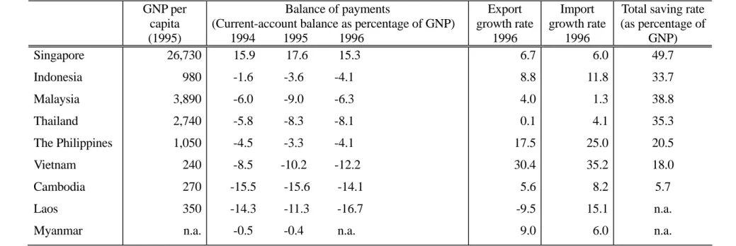
The currency crisis in Thailand was brought partly because of macroeconomic instability. In other words, problems with balance of international payments in the macroeconomy, more precisely, external current account deficits, helped to depreciate the exchange rate in a short term starting in July 1997. The devaluation of Thai baht was brought partly due to economic fundamentals. That is, current account deficits accounted for 8.1% of GDP in 1996. The level of current account deficits was worse than that of Mexico which experienced the currency crisis in 1994 (Table 1).
We will explain the determinants which brought current account deficits in balance of payments to Thailand. Thailand had the deficits because its export growth rate, which had been favorable up until 1995, slowed down, reaching nearly zero in 1996. Deterioration of
economic fundamentals forced the country to devaluate its currency to recover export competitiveness in the currency market.
By the way, even with declining exports and worsening trade balance, deterioration of overall balance can be avoided by a government policy through maintaining high interest rate and capital-account surplus. However, falling export competitiveness, i.e., deterioration of economic fundamentals, cannot be supported by such policy in the long term. Thus, Thailand's government was forced to give up capital inflows based on high interest rate policy.
Certainly, exports rose by 6.2% in July 1997 from the previous year in Thailand, as a result of simplified export procedures. Part of the growth may be a result of depreciation of the exchange rate. For example, in the Philippines too, exports increased by 22.8% in first eight months of 1997, compared to the same period in the previous year (National Statistics Office). The main factor for the increase is depreciation of the exchange rate. However, that would not lead to improvement of the export structure in the medium and long term.
Next, it is necessary to examine why Thailand's export competitiveness declined. To that end, the mechanism of export growth since the late 1980s will be illustrated. The mechanism of the export growth was export-oriented industrialization through attracting foreign capital. Export processing zones played an important role to attract foreign capital. Thus, Thailand's economy experienced growth through establishing export processing zones, attracting foreign capital, and increasing exports. The export processing method generated three bottlenecks: shortage in skilled labor, undeveloped infrastructure, and underdevelopment of supporting industries. The most serious problem of them was the shortage in skilled labor. The cheap wage structure due to surplus workers, which was one of the largest incentives for foreign companies to enter into Thailand, started to collapse. Especially for Thailand, shortage of engineers and managers were critical. Thus, inflows of foreign direct investment into Thailand dropped substantially.
The decline of foreign direct investment into Thailand was also substantial when looking at the first quarter record of 1997 (Bank of Thailand). For example, in the manufacturing industry foreign direct investment dropped by 65% from the previous year, and the overall direct investment decreased by 32%. When looking at investment from each country, while Japan increased its direct investment, the U.S. and Singapore reduced their investment significantly.
The above paragraphs discussed economic fundamentals. Yet, we cannot deny that
the foreign exchange market and the stock market have the technical aspect (psychological aspect) of the price movements too. Thailand's stock market reached a peak in 1994, and since then it maintained the downward trend. The stock price fall was accelerated by the currency crisis.
3. Portfolio and business cycles
Alfredo (1992) showed that GDP movements have chaos as well as cycles . Similarly, Grandmont (1985) proved existence of cycles and stable periodic orbits. Here we will apply the Overlapping Generations Model (OLGM) to showing that level of GDP depends on a expected value of stock prices. Next, we will examine a case in which households engage in portfolio investment. In other words, we consider the case when households invest not only in stocks markets, but also in markets of primary commodities such as crude oil. In the latter case, GDP movements depend on changes in both stock and commodity prices. This model is based on Diamond (1965).
(1) Consumer: Utility function (Ut) in period t depends on consumption (ct) in period t and consumption (c ) in period t+1 as indicated by the following simple utility function. That is, we assume
1 + t Ut = cty + ct + + log log 1 0 1 ρ
where y denotes young and o denotes old. Budget constraints in period t and period t+1 are c s w c r t t t t t + = = + + + , ( ) 1 1 1 st )
respectively, where st is savings of representative household, wt is the wage rate in period
t, and rt+1is the interest rate in period t+1. Condition of utility maximization is
1/ct = +(1 rt+1) /ct+1(1+ρ
Therefore, solving for st, we have,
st = wt/ (2 + ρ ) (1) (2) Firm: Consider the following production functions per person
y Y L f k k K L t t t t t t t ≡ / = ( ) , ≡
where Y is total output, K is capital stock, and L is labor. Now suppose the Cobb-Douglas production function which takes the form of f (kt) = A k . The company's
t t t
α
t
profit maximization is subject to = rt f ‘(kt) = α−1 (2) t Ak wt = f(kt)– k + f ‘(kt)= (1 – α)Aktα (3) (3) Market equilibrium: The condition is
rtKt + wtLt = Kt+1 – Kt + y t + t L c 1 0 − t t L c and we obtain Kt+1 =stLt Therefore, kt+1 = st / (1 + ) n (4) From Equations (1), (3), and (4), we have
kt+1 = (1 – α)Aktα / (2 + ρ (1 + ) (5) ) n
(4) Arbitrage condition (no arbitrage): Here, suppose that stock price in period t is Pt, and the expected stock price in period t+1 is Pe
t+1. Arbitrage condition is e t (6) t t P P r / 1+ +1 = +1
After having the above equations, substitute kt in the Cobb-Douglas production function with kt+1by Equation (5), and then substitute the kt+1 with rt+1 by Equation (2). Finally, substitute the rt+1with P / Pt by Equation (6), and we obtain
e t 1+ yt = 1 1 1 1 1 ) 1 ( ) 1 )( 2 ( + − ⎪⎭ ⎪ ⎬ ⎫ ⎪⎩ ⎪ ⎨ ⎧ − ⎟⎟ ⎠ ⎞ ⎜⎜ ⎝ ⎛ − + + α α α ρ t e t P P A n (7) the function showing that production per person depends on the stock price.
Next, consider the case of portfolio (asset selection). Suppose, for example, that shares of stock and crude oil are δ and 1-δ, respectively.
Then,
P qt = Plt(δq)+Pmt
{
(1−δ)q}
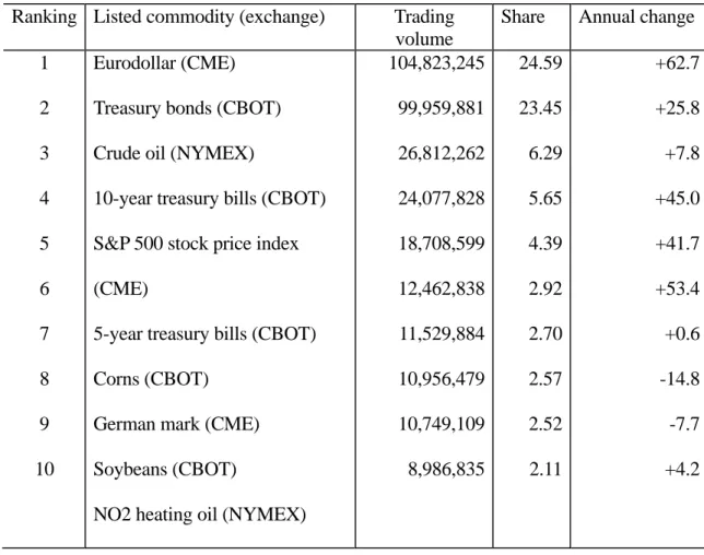
where P and P are prices of stock and crude oil in period t, respectively, and q denotes total purchase unit. Portfolio is indicated by the percentage of volume such as 23.45% for treasury bond and 6.29% for crude oil, as shown in Table 2. Similarly, for period t+1, it is assumed as t λ mt P qt P q P
{
q}
e t e mt e +1 = l +1(δ )+ +1 (1−δ) Therefore, 7y n A P P P P t t e mt e t mt = + + − + − + − − ⎛ ⎝ ⎜ ⎞ ⎠ ⎟ ⎧ ⎨ ⎪ ⎩⎪ ⎫ ⎬ ⎪ ⎭⎪ + + − ( )( ) ( ) ( ) ( ) 2 1 1 1 1 1 1 1 1 1 1 ρ α α δ δ δ δ α l l
That is, cyclical movements depend on the expected prices of stocks and crude oil in the future period.
4. Theorem of unpredictability
The analysis in the previous section showed that GDP depends on movements of stock prices and commodity prices. And it is widely known by stock price analysis that stock prices have cycles, such as the ones called "Elliott Waves" or "Reverse Watch Curve." Stock prices movements can be explained partly by these technical analysis since investors behaves according to them.
Elliott published "Elliott Wave Principle" (Financial World, 1939), proposing categories such as the Super Cycle (approximately 50 years and similar to Kondratieff Wave), the Cycle (nearly 10 years and similar to Juglar Cycle), and the Primary Cycle (1 - 4 years, similar to Kitchen Cycle). He suggested that in the Super Cycle one cycle consists of two waves, one upward wave and one downward wave, the Cycle consists of has eight waves, three downward waves and five upward waves, and the Primary Cycle consists of thirty-four waves, thirteen downward waves and twenty-one upward waves. They are based on Fibonacci numbers which was discovered by the Italian mathematician, Fibonacci.
Now, using the psychological line, examples of psychological cycles of exchange rate of Japan’s currency yen, the Nikkei Average price of Japan’s stocks, and a gold price will be illustrated. We explain the psychological line as follows. First, we identify whether every average monthly gold price for the last twelve months, increased decreased, or unchanged compared with that of the previous month. Second, we count the number how many months out of the last twelve months the monthly prices increased. Third, we calculate the ratio of the number of the increased months to twelve: the ratio is zero (= 0 / 12) when the number of the increased months is zero, it is 100 (= 12 /12) when the number is 12, and it is 50 (= 6 / 12) when the number is 6. This index indicates psychological cycles, and will change over time. The psychological line of a gold price fluctuates periodically. Besides, as shown in Section 4, periodic cycles cannot be observed by a graph. Similar psychological cycles can be observed in the Nikkei Average price of Japan’s stocks for the
same period and the exchange rate of the yen.
Thus, it is known that stock prices have cycles, and it is worth noting that numbers which are the bases of the cycles are prime numbers.
Next, we look at the "reverse watch wave." Phases of reverse watch wave are: 1. Positive signal: When volume is increasing and stock prices touch the bottom. 2. Buy signal: When volume is increasing and stock prices turn to move upward.
3. Consistent buying: When volume remains at the same level and only stock prices are rising.
4. Wait to buy: When volume starts to fall and only stock prices are rising. 5. Watch signal: When volume is falling and stock prices are unchanged. 6. Sell signal: When volume is falling and stock prices turn to move downward.
7. Consistent selling: When volume stops to fall and stock prices continue to drop sharply. 8. Wait to sell: When stock prices continue to fall but volume is increasing. The above cyclical phases are seen in the stock market.
Now, assuming that stock price movements draw the polygonal "Reverse Watch Curve" with n sides, according to the group theory it is isomorphic to:
H = Z = {n 0, 1 , --- , n } For example, when n=3
Z = {3 0, 1 , 2 }
and if 0= price stability, 1 = price increase, and 2 = price decrease, then the order of price stability, increase, decrease, and stability, increase, decrease will be repeated. The Reverse Watch Curve is considered to have n=6, and stock prices repeat the cycle of
Z6 = {0, 1 , 2 , ,3 4 , 5}
unless external conditions change. Then, application of the theorem of the group theory has significant agreement with business cycles.
"Theorem 1: Every group of a group generates a cyclic subgroup of the group." This implies that stock prices contain cycles in their movements. Hence, if spectrum analysis is performed on stock price movements, cycles can be found. As long as external economic environment is unchanged, stock prices repeat the same cyclical movements.
Consequently, it is possible to predict stock price movements. This is so called the Box market.
As for cycles in stock price movements, the following theorem also has agreement.
"Theorem 2: While the foregoing n is called as order, every group of prime order is cyclic."
Accordingly, it is possible that stock prices have cycles of prime numbers such as three months or five months.
Now, go back to the argument of GDP movements. As said in Section 2, assume that GDP depends on prices of stocks and primary commodities (such as prices of crude oil). Then, suppose that stock prices have a cycle of three months (Z3), and oil prices have a cycle of five months (Z ). Now, GDP movements follow 5
Z 3 × Z5
These movements are illustrated in Figure 1. It means that GDP has a cycle of 3 × 5 = 15 months. However, actual GDP movements are not systematic waves so as to go up, down, and up. As shown in Figure 1, prices appear to move completely randomly. Thus, it is difficult to predict these movements.
The foregoing paragraphs explained the case where stock prices and commodity prices have cycles of primary numbers. The following paragraph will examine the case where cycles are not in primary numbers.
Order of Z n × Z follows the theorem below: m
"Theorem 3: For instance, when the cycle of stock prices is 6 months (n) and that of oil prices is 8 months (m), GDP cycle would be the least common multiple of 6 (=n) and 8 (=m), which is 24 months."
Implication of the theorem is as follows. Suppose, for example, that peaks and bottoms of business cycles are determined for GDP data. Here, while one cycle consists of 24 months, a spectrum analysis would show 6- and 8-month cycles. And, GDP movements do not show periodic peaks and bottoms. That is, determination of economic peaks and bottoms from GDP is difficult.
5. The existence of negative bubble
In examining bubble, assume a stock M (useless pieces of paper). Bubble is assets with no substantial use. Here, the price of M in term t is denoted as Pt. Thus, when Bt' is
the value of the bubble, we have Bt'= M pt
However, bubble is always found in speculative products. Therefore, we introduce the concept of optimistic (bull) and pessimistic (bear) outlook observed by market participants. In any kind of market, popularity determines the price of the bubble, pt. We denote popularity per person as bo. Then, the total value of the bubble when accounted for
popularity (Bt) is
= Bt' + , (8)
t
B b0Lt
(where Bt' = Mpt).
Here, arbitrage condition is, as given earlier, 1
1/ 1 + + t = + t
t P r
P (9) and from Equation (1) and (2), we have
( ) 1 0 1 1 b b n n r b b t t t t + − − = − + + (10) where bt = Bt /Lt
Hence, under the steady state of bt+1- bt = 0, we get
n
rt+1 = (11)
Assuming the Cobb-Douglas production function, we have ) 1 /( 1 1 − + ⎟ ⎠ ⎞ ⎜ ⎝ ⎛ = α αA n kt (12) Next, consider market equilibrium. From arbitrage condition and definition of bubble, Bt' = Mpt, we have
Bt'= +(1 rt)Bt′−1
Adding the both sides of this equation to the market equilibrium condition given in Section 2, we get Kt+1−St +Bt'= +(1 rt)(Kt −St−1+ ′Bt−1) Thus, we have (13)
{
1/(1 )}
( 0) 1 n s b b kt+ = + t − t +Now, consider a household and a firm. Assuming more general utility function,
U c cty to ct c y t o ( , ) ( ) ( ) ( )( + − + − = − + − + 1 1 1 1 1 1 1 θ θ θ θ ρ) we have ⎭ ⎬ ⎫ ⎩ ⎨ ⎧ + + + = + −− 1 ) 1 ( ) 1 ( / (1/ ) ) / 1 ( 1 1 θ θ ρ t t t r w s (14) Also, from condition of company's profit maximization, we obtain
(15) α
α t
t Ak
w =(1− )
Therefore, from Equation (11) to (15), we can get a BB curve with geometric locus of bt−1- bt= 0, ) 1 /( 1 0 ) / 1 ( ) / 1 ( 1 (1 ) 1 ) 1 /( ) 1 ( ) 1 ( − − − ⎟⎠ ⎞ ⎜ ⎝ ⎛ + − + + + + − = α θ θ α α ρ α A n n b n Ak b t t (16)
This BB curve has
db dk d b dk t t t t >0 <0 2 2 ,
Also, deriving a KK curve with geometric locus of kt+1- kt = 0 from Equation (13),
we have 1 (1/ ) (1/ ) (1 ) 0 1 ) 1 /( ) 1 ( ) 1 ( b k n n Ak b t t t − + + + + + − = − θ α− θ ρ α (17) This curve has a point,
k A z n o = − + ⎧ ⎨ ⎩ ⎫ ⎬ ⎭ − α( α) α ( ) /( ) 1 1 1 1
as illustrated in Figure 2. Here, we set =(1+ )1−(1/θ)/(1+ρ)−(1/θ) +1.
n z
Then, the intersection of the BB curve and the KK curve can be find, and condition for the bubble, bt, to be negative is
{
}
[
]
b n A z n n o < ⎛ ⎝ ⎜ ⎞ ⎠ ⎟ + + + − − − α α α α α θ 1 1 2 1 1 1 1 2 1 /( ) ( / ) ( ) ( ) tIn other words, when individuals become more pessimistic beyond certain level, a negative bubble will be generated. This is illustrated in Figure 3.
Suppose P is the fundamental value, bt is the bubble, and Pt is the price affected by the bubble. Then,
ft
Pt = Pft +b
holds. In the following paragraphs, we calculate the value of P and Pt and find the case when the value of the bubble, bt is negative.
ft
First, we calculate the fundamental value. At this time, assumptions under rational expectations (assumptions of Martingale are also used) are critical. This would be
[
]
Pft E R I r i K t i t = + = ∞ +∑
+ 0 1 1 / (1 )where R is dividend, It is available information in term t, and r is the discount rate. Now, assuming k R d (constant) , t k+1 = 12
we have
Pft = / rd
(refer to Tirole (1985)) .
Next, consider the case when rational expectations do not hold. We put it as
Pte uE Pt I
t
+1 = ( +1 )
where u is divergence from the fundamental value and u > 0. At this time, Pt =d / (1+ −r u)
and, we have
bt =d u( −1) / (1+ −r u)r
Hence, condition for producing negative bubble is 0< <u 1, u> +1 r
Considering intersectional condition, when 0< <u 1
holds, negative bubble can exist.
6. Conclusions
We have theoretically obtained the three following conclusions. First, business cycles depend on prices of stocks and primary commodities such as crude oil. Second, stock prices and oil prices generate psychological cycles with different periods. Third, contrary to the Tirole conclusion [1985], there exist cases of “negative bubble” under certain conditions. Integrating the above results, we can find a role of a government.
For example, suppose a stock price cycle of three months and an oil price cycle of five months. These two cycles generate a fifteen month cycle. At this time, after positive bubble is generated in the fifteen-month cycle, negative bubble develops. Accordingly, when negative bubble is large, a government should take a policy to shift the cycle by intervening the market.
Moreover, assume that there is a seven-month cycle of treasury bond prices on top of the stock and oil price cycles. Then, the business cycle becomes 105 months. The negative bubble is likely to become larger reflecting the longer duration of the cycle. In an economy which continues to grow rapidly, a positive bubble (i.e., speculation) is continuously observed phenomena, and as a rebound a negative bubble becomes larger. One of important roles of governments is to shift these cycles to avoid a deep recession, or a great
Tirole, J., "Asset Bubble and Overlapping Generations," Econometrica 53 (1985), 1071-1100.
Diamond, P., "National Debt in a Neoclassical Growth Model," American Economic Review, 55 (1965), 1126-1150.
Grandmount, J.M., "On Endogenous competitive Business Cycles," Econometrica, 53 (1985), 995-1045.
Alfred, M., Chaotic Dynamics, Cambridge University Press, 1992.
<References >
depression when a negative bubble is large. Combination of a negative bubble and psychological cycle will let investors rush to sell currency. So that intervention is necessary to avoid the panic selling in the market.
15
Table 1: Economic Indicators of the ASEAN (Unit: %)
GNP per
capita (1995)
Balance of payments
(Current-account balance as percentage of GNP) 1994 1995 1996 Export growth rate 1996 Import growth rate 1996
Total saving rate (as percentage of GNP) Singapore Indonesia Malaysia Thailand The Philippines Vietnam Cambodia Laos Myanmar 26,730 980 3,890 2,740 1,050 240 270 350 n.a. 15.9 17.6 15.3 -1.6 -3.6 -4.1 -6.0 -9.0 -6.3 -5.8 -8.3 -8.1 -4.5 -3.3 -4.1 -8.5 -10.2 -12.2 -15.5 -15.6 -14.1 -14.3 -11.3 -16.7 -0.5 -0.4 n.a. 6.7 8.8 4.0 0.1 17.5 30.4 5.6 -9.5 9.0 6.0 11.8 1.3 4.1 25.0 35.2 8.2 15.1 6.0 49.7 33.7 38.8 35.3 20.5 18.0 5.7 n.a. n.a. Source: Asian Development Bank's Economic Outlook (1997), (Asian Development Bank)
Table 2: Commodity Ranking by Trading Volume (1994)
(Units: pieces, %) Ranking Listed commodity (exchange) Trading
volume
Share Annual change 1 2 3 4 5 6 7 8 9 10 Eurodollar (CME) Treasury bonds (CBOT) Crude oil (NYMEX)
10-year treasury bills (CBOT) S&P 500 stock price index (CME)
5-year treasury bills (CBOT) Corns (CBOT)
German mark (CME) Soybeans (CBOT)
NO2 heating oil (NYMEX)
104,823,245 99,959,881 26,812,262 24,077,828 18,708,599 12,462,838 11,529,884 10,956,479 10,749,109 8,986,835 24.59 23.45 6.29 5.65 4.39 2.92 2.70 2.57 2.52 2.11 +62.7 +25.8 +7.8 +45.0 +41.7 +53.4 +0.6 -14.8 -7.7 +4.2 16
Figure 1. Cycles with 3 periods and 5 periods
0 1 2 3 4 5 6
Z
3Z
5 0 0 0 ・ 1 1 2 ・ 2 2 4 ・ 0 3 3 ・ 1 4 5 ・ 2 0 2 ・ 0 1 1 ・ 1 2 3 ・ 2 3 5 ・ 0 4 4 ・ 1 0 1 ・ 2 1 3 ・ 0 2 2 ・ 1 3 4 ・ 2 4 6 0 0 0 ・ 1 1 2 ・ 2 2 4 ・ 0 3 3 ・ 1 4 5 ・ 2 0 2 ・ 0 1 1 ・ 1 2 3 ・ 2 3 5 ・ ・ 17Figure 2. KK Curve
KK=
KK
k
0b
0b
tk
t 0 ) 1 ( ) 1 ( b k n Z Ak b t t t − + + − = α α α α α − ⎭ ⎬ ⎫ ⎩ ⎨ ⎧ + − = 1 1 0 ) 1 ( ) 1 ( n Z A k 18Figure 3. Existence of Negative Bubbles