博
士
論
文
Research for Tsunami Measurement Based on 3D Image
Measurement Technique
福岡工業大学大学院工学研究科
知能情報システム工学専攻
伊 浩
要旨
津波被害を減らすためには、津波の早期発見が必要である。本研究の目的は、 陸上に設置したカメラから 5km~20km 先の海面の変化を監視することである。 本論文では、津波計測のための 3 次元画像計測技術を用いた遠距離海面高度 計測システムの構築について紹介する。まず、広範囲の海面を計測するために、 パン・チルト・ステージを用いてカメラの角度を制御する。また、計測精度を向 上するために、特徴が既知のスケールポールを使用して、カメラの固有パラメー タおよび計測システムの外部パラメータを較正する手法を提案した。また、海波 を抽出するために、領域分割法と動的閾値法を用いた波自動抽出手法を提案し た。最後に、海波の平均高さに基づく海面の高さを算出する手法を提案した。 本論文は 5 つの章で構成されている。第 1 章では、本論文の背景と既存の津 波計測手法について説明し、3 次元画像処理技術を用いた津波計測の考え方を提 案する。その後、本研究の目的と本論文の構成を述べる。 第 2 章では、遠方海面計測のためのカメラシステムのキャリブレーション方 法について述べる。まず、両眼立体視の理論とカメラキャリブレーション方法を 説明し、遠距離のキャリブレーションの困難性を述べる。その後、提案したキャ リブレーション手法を述べる。 第3 章では、海波の抽出方法について述べる。まず、遠距離の海波抽出の困難 性を説明し、提案した領域分割法と動的閾値法を用いた波の自動抽出法を述べ る。その後、ステレオ画像上の海波のマッチング方法について述べる。まず、対 応点をそれぞれマッチングすることの困難性を説明し、この問題に対する解決 策を述べる。 第4 章では、検証実験の方法、実験結果及び考察を述べる。まず、実験条件と 実験方法を紹介し、その後実験結果について説明し、考察を述べる。 第5 章では、本論文のまとめと今後の課題について述べる。Abstract
In order to reduce the loss of lift in disasters, it is necessary to construct a tsunami measurement system. Our purpose is to monitor the change of sea levels of 20 km using by two cameras installed on the seashore.
In this paper, we construct the measurement system of long distance sea-level height based on 3-D image measurement technique. First, in order to measure a wide range of the sea surface, we can use the pan and tilt stage to rotate cameras in this system. In order to improve the accuracy of the tsunami measurement system, we propose a long distance calibration method of camera measurement system that uses the standard scale pole to calibrate intrinsic and extrinsic parameters of cameras system. Then, we proposed a dynamic threshold method in blocks to extract the sea waves automatically. Finally, we propose a sea level calculation method based on average value of wave heights.
This paper consist of five chapters. In the Chapter 1, we explain the background of this paper and tsunami measurement methods, In addition, we proposed our approach of tsunami measurement system with 3-D image measurement technique. Then, we introduce the system and explain the purpose of this research.
In the chapter 2, we propose the calibration method of long distance 3-D image measurement system. First, we illustrate the theory of binocular stereoscopic vision and camera calibration. Then we explain the method of camera calibration.
In the chapter 3, we introduce the extraction method of sea wave. First, we illustrate the difficulties of long distance sea wave extraction and then we proposed a dynamic threshold extraction method for long distance image. Then, we introduce the difficulties of corresponding point matching. Finally, based on feature matrix, we propose a method of matching point and show the results of this method.
In the chapter 4, we describe the experimental conditions, the experimental results and consideration.
In the chapter 5, we summary the work in this paper and give an outlook of the future work.
Contents
Chapter1 Introduction... 1
1.1 Analysis of tsunami characteristics and tsunami disaster ... 2
1.2 The meaning of wave height measurement and the existing measurement methods ... 6
1.3 3-D image measurement technology ... 11
1.4 The purpose of our research and structure of this paper ... 15
Chapter2 Calibration of long distance 3-D image measurement system ... 16
2.1 The theory of binocular stereoscopic vision ... 17
2.2 The existing calibration method ... 25
2.3 The improved calibration method ... 27
2.4 Calibration experiments ... 30
2.5 Summary ... 38
Chapter3 Image processing ... 39
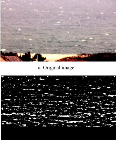
3.1 Difficult of sea wave extration ... 40
3.2 Sea wave extraction ... 45
3.4 Experiments and results ... 53
3.5 Summary ... 57
Chapter4 Experimental results and consideration ... 58
4.1 Proposed sea wave height measurement system ... 59
4.2 Experimental conditions ... 61
4.3 Measurement of the height of sea level ... 62
4.4 Experiments and results ... 64
4.5 Summary ... 92
Chapter5 Conclusions... 93
References ... 95
Research Published ... 100
Figure 1.1 Tsunami propagation ... 3
Figure 1.2 Wind-generated waves ... 4
Figure 1.3 Tsunami in Miyako ... 5
Figure 1.4 Measurements along coast ... 7
Figure 1.5 Measurements in open sea area ... 7
Figure 1.6 Dart system ... 9
Figure 1.7 TOF system ... 12
Figure 1.8 The system of pattern projection method... 12
Figure 1.9 Stereo vision method ... 13
Figure 1.10 Ideal stereo vision system ... 14
Figure 2.1 Images coordinate and the image plane coordinate ... 18
Figure 2.2 Theory of pinhole model ... 19
Figure 2.3 Binocular stereo vision system in the ideal model ... 22
Figure 2.4 The measurement theory of x and y axis ... 23
Figure 2.5 The usual model of binocular stereo vision system ... 24
Figure 2.6 Calibration block of DLT method ... 25
Figure 2.7 Mapping relations between the images coordinate with the world coordinate ... 26
Figure 2.8 Calibration model ... 27
Figure 2.9 The sea area in Shikashima ... 30
Figure 2.10 Image at 12:00 ... 31
Figure 2.11 Images at 12:30 ... 31
Figure 2.12 Images at 13:15 ... 31
Figure 2.13 The images of calibration in Shikashima ... 32
Figure 2.14 Sea area in Shigu ... 33
Figure 2.15 Hollow plastic bar for calibration ... 34
Figure 2.16 Calibration image in Shigu ... 34
Figure 2.17 Verification images in Shigu ... 35
Figure 2.18 Sea area in Tsuyazaki ... 36
Figure 2.19 Calibration Images in Tsuyazaki ... 37
Figure 3.1 Extract image with Otsu threshold ... 41
Figure 3.2 Extract image with adaptive threshold ... 43
Figure 3.3 The sawteeth in image ... 44
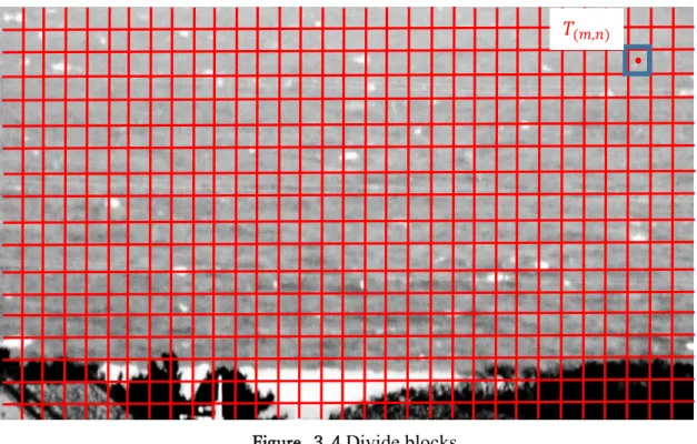
Figure 3.4 Divide blocks ... 45
Figure 3.5 Optimum block threshold method ... 47
Figure 3.6 Comparison of the results ... 47
Figure 3.8 Select sea wave ... 49
Figure 3.9 Template Matching ... 50
Figure 3.10 SIFT matching ... 51
Figure 3.11 The feature of sea wave ... 52
Figure 3.12 Extraction result (1) ... 54
Figure 3.13 Matching result (1) ... 55
Figure 3.14 Extraction and matching result (2) ... 56
Figure 4.1 Measurement System ... 59
Figure 4.2 Flow chart of sea-level height measurement ... 60
Figure 4.3 Measurement system ... 61
Figure 4.4 The change of sea-level height ... 62
Figure 4.5 Experiment places ... 64
Figure 4.6 Images in Shigu at 6:48 ... 65
Figure 4.7 Calculation of the height of sea level at 6:48 ... 66
Figure 4.8 Image in Shigu at 7:49... 67
Figure 4.9 Calculation of the height of sea level at 7:49 ... 68
Figure 4.10 Image in Singu at 8:50 ... 69
Figure 4.11 Calculation of the height of sea level at 8:50 ... 70
Figure 4.12 Image in Singu at 9:51 ... 71
Figure 4.13 Calculation of the height of sea level at 9:51 ... 72
Figure 4.14 Image in Singu at 10:52 ... 73
Figure 4.15 Calculation of the height of sea level at 10:52 ... 74
Figure 4.16 Image In Singu at 11.53 ... 75
Figure 4.17 Calculation of the height of sea level at 11:53 ... 76
Figure 4.18 Image in Singu at 12:53 ... 77
Figure 4.19 Calculation of the height of sea level at 12:53 ... 78
Figure 4.20 Image in Singu at 13.54 ... 79
Figure 4.21 Calculation of the height of sea level at 13:54 ... 80
Figure 4.22 Image In Singu 14:55 ... 81
Figure 4.23 Calculation of the height of sea level at 14:55 ... 82
Figure 4.24 Image in Singu at 15:56 ... 83
Figure 4.25 Calculation of the height of sea level at 15:56 ... 84
Figure 4.26 Image in Singu at 16:57 ... 85
Figure 4.27 Calculation of the height of sea level at 16:57 ... 86
Figure 4.28 Image in Singu at 17:58 ... 87
Figure 4.30 Experiment result in Singu on March 8 ... 89
Figure 4.31 Experiment result in Singu on March 9 ... 90
Figure 4.32 Experiment result in Singu on March 10 ... 90
Figure 4.33 Experiment result in Singu on March 14 ... 91
Figure 4.34 Experiment result in Singu on March 15 ... 91
Table 2.1 Camera parameters ... 21
Table 2.2 The result of calibration in Shikashima ... 32
Table 2.3 The error of calibration in Shikashima ... 33
Table 2.4 The result of calibration in Shigu ... 35
Table 2.5 The error of calibration in Shigu ... 36
Table 2.6 The result of calibration in Tsuyazaki... 37
Table 2.7 The error of calibration in Tsuyazaki... 37
Table 3.1 Gaussian convolution kernel ... 42
Table 3.2 Result of matching image (1) ... 55
Appendices-Sign in paper
A: The sum of all the pixels of sea wave.
𝐴𝑆𝑖𝑗: The similarity of the area. 𝑏: The length of base line.
C: The ratio of perimeter to area.
𝐶(𝑖,𝑗): The cross-correlation constraint at the point(𝑖, 𝑗). 𝐶0(𝑡), 𝐶1(𝑡): The two classes separated by a threshold t. 𝐶𝑆𝑖𝑗: The similarity of the curvature.
𝑑𝑥, 𝑑𝑦: The physical dimensions of one pixel in the X-axis and Y-axis. 𝐷𝑖𝑠𝑡𝑖𝑗: The similarity of the feature vector.
𝑓: The local length of camera.
𝑓(𝑖, 𝑗): The gray value at the point(𝑖, 𝑗) in the input image. 𝑔: The standard acceleration due to gravity.
ℎ: The height from the sea surface to the seafloor. 𝐻(𝑖,𝑗): The Gaussian convolution kernel in point(𝑖, 𝑗). 𝑖: Image coordinate in 𝑥 direction.
𝐼(𝑚,𝑛), 𝑅(𝑚, 𝑛): The gray value at the point (m, n). 𝐼̅, 𝑅̅: The average gay value with block size M × 𝑁. 𝑗: Image coordinate in 𝑦 direction.
𝐿𝑖: The length from the point Pi to point Qi. 𝑀1: The internal parameter matrix of the camera. 𝑀2: The external parameter matrix for the camera. 𝑛𝑖: The number of the gray value 𝑖.
𝑂(𝑖, 𝑗): The gray value at the point(𝑖, 𝑗) in the output image.
P: The sum of all the pixels of the perimeter of sea wave.
𝑝: The ratio of left-(x, y) width per block width. 𝑝𝑖: The probability of each gray value.
𝑃𝑀: The 3×4 projection matrix. 𝑃𝑆𝑖𝑗: The similarity of the perimeter.
𝑞: The ratio of bottom-(x, y) width per block width. 𝑟: The distance from each pixel to center point.
R: The rotation matrix.
𝑇(m,𝑛): The threshold in block (m, n). 𝑡(i,j): The threshold of point(𝑖, 𝑗).
𝑇𝑥, 𝑇𝑧, 𝑇𝑧: The element of translation matrix (𝑢, 𝑣): The point position in pixel coordinates. (𝑢0, 𝑣0): The principal point of camera. 𝑣: The speed of Tsunami.
V: The feature vector.
𝑉𝐿: The left feature matrix.
VR: The right feature matrix
(𝑥0, 𝑦0): The center point of image. (𝑥𝑖, 𝑦𝑖): The point coordinate in the image.
𝑋𝑤, 𝑌𝑤, 𝑍𝑤: The coordinate in 3-D world coordinates. 𝑋𝑐, 𝑌𝑐, 𝑍𝑐: The coordinates in the 3-D camera coordinates 𝑌𝑖: The height value of sea wave.
𝑌𝑆𝑖𝑗: The similarity of the position.
𝛼: The angle of rotating toward the z_axis. 𝛽: The angle of rotating toward the y_axis. 𝛾: The angle of rotating toward the x_axis. 𝛿2(𝑡): The variance of threshold t.
𝜔0(𝑡), 𝜔1(𝑡): The probabilities of the two classes separated by a threshold t. 𝜇0(𝑡), 𝜇1(𝑡): The average gray of 𝐶0(t) class, 𝐶1(𝑡) class.
1
Chapter1 Introduction
Tsunami, one of the most dangerous natural disasters, damages the coastal countries. Tsunami occurs frequently in recent years. Thus, it is necessary to detect the tsunami before it reaches the shore in 15 to 20 minutes. Comparing with typical tsunami prediction methods, our lab has proposed a method based on 3-D image measurement technique to detect the long distance sea surface. In order to achieve the purpose of the tsunami forecast eventually, we must overcome all kinds of problems of long distance. This system monitors the range of sea waves which are more than 20km.
In this chapter, first, we will introduce the purpose of our research, the characteristics of the tsunami and the existing methods of tsunami forecast. Then, we introduce the 3-D image measurement technique. Finally, we introduce the research significance of this research and the structure of the system.
2
1.1 Analysis of tsunami characteristics and tsunami disaster
Tsunami is a series of huge waves that can cause great devastation and loss of life when reaching coasts. Tsunami is caused by the underwater earthquake, a volcanic eruption, a sub-marine rockslide, or, more rarely, by an asteroid or meteoroid crashing into in the water from space. Most tsunamis are caused by underwater earthquake, but not all underwater earthquakes cause tsunamis - an earthquake is over about magnitude 6.75 on the Richter scale to cause the tsunami [1]. About 90 percent of all tsunamis occur in the Pacific Ocean.
Many tsunamis are detected before they hit the land, and the loss of life can be minimized. With the use of modern technology, including seismographs (which detect earthquakes), we can computerized offshore buoys that can measure changes in wave height, and a system of sirens on the beach to alert people of the potential danger of tsunami.
When considering how tsunami waves propagate, or travel across the ocean, it is important to understand wave behavior. Before discussing tsunami waves, we know the definition and characteristics of the wave. Comparing wind-generated waves, tsunami waves are useful for understanding the force, scope and potential danger of large tsunamis.
Using data from past tsunami events and known wave characteristics, scientists have developed models for calculating tsunami travel times to deliver warnings to communities that may be impacted by the tsunami. These models make use of complex data based on the size and location of an earthquake, the depth of the ocean determined by bathymetric measurements, the distance to a given location, the shape of the coastline in impacted zones, and past run-up heights.
Scientists of the tsunami warning center have developed some models to predict the arrival times of tsunami for the certain high-risk locations. When an earthquake of magnitude 6.75 or higher magnitude generates along a coastal area, warning centers may be able to warn communities of an impending tsunami and estimate when the first wave will arrive.
In the early stage, huge waves cannot be observed when the tsunami is far from coast and the propagation speed can be very fast. With the tsunami coming to near shore areas, obvious huge waves can be noticed and tsunami propagation velocity will slow down. Figure 1.1 shows the relations between depth, velocity and the wave length. This phenomenon stems from the relationship of tsunami propagation velocity and sea depth in the equation (1.1) [2].
3
v = √𝑔ℎ (1.1)
(https://www.senat.fr/opecst/english_report_tsunami/english_report_tsunami2.html) Figure 1.1 Tsunami propagation
Where, v is the propagation velocity of tsunami, g is the gravitational acceleration, and h is the depth of the sea. It is difficult to detect the tsunami when the height of the sea waves is low and the propagation velocity is high in the early stage [3].
Waves are a disturbance that propagates, or travels, through space and time transferring energy from one point to another. Waves can be electromagnetic or mechanical. The basic parts of any type of waves are same, although waves differ in their characteristics.
The state of equilibrium is the state when the system is in balance. The disturbance makes the system out of equilibrium. All systems try to return to equilibrium after the disturbance.
Gravity is the force that attempts to restore water molecules to equilibrium when they are disturbed by the wave energy.
The equilibrium of ocean water is disturbed by the gravity of the moon and the sun, which produce the tides. Other disturbances include tsunami triggers, wind and human and animal activity.
There are four basic types of water waves: tides, seiches, wind-generated waves, and tsunamis waves.
Tides are the sea level rise and fall caused by the combined gravity of the moon and the sun. The seiche is a standing or stationary wave oscillating in an enclosed body of water such as a bay, lake or reservoir often caused by an earthquake, wind or tsunami. A
4
seiche looks like waves that slosh back and go forth from one end of a bay to another. Two propagating waves traveling in opposite directions combine to form the standing wave.
Most ocean waves are generated by wind. As the wind blows across the surface of the water, it pushes on the surface of the water forming waves. Wind can create waves of different sizes, from small capillary or ripple waves, to large swells. Strong winds and storms can produce chops and swells. Wavelengths vary from centimeters to 90 meters high (300 feet) as follow in the Figure 1.2 [4].
As the wind blows on the surface, the energy of the wave reaches a certain known depth into the water and the depth of influence, which is equal to one half of the wavelength. The motion of the water particles decreases as depth increases, until the depth of influence is reached.
In deep water, wind waves cause water particles to move in a circular motion. There is a common misconception is that wind waves propel a boat or an object forward on the surface of the water. Because water particles return to the same position approximately as the energy passes through, an object on a wave does not move forward with the wave energy, but it returns to the same general area.
(https://trestlessurfcrowd.wordpress.com/tag/capistrano-beach/) Figure 1.2 Wind-generated waves
5
As wind-generated waves approach a shoreline, and the depth of the water decreases, the height and amplitude of the wave increases until the wave breaks due to gravity, which is popular for surfers [5].
Tsunami waves differ from wind-generated waves which shouldn’t be surfed. When tsunamis produce, the water is displaced by an earthquake, landslide, or volcanic activity , they can generate waves that travel in all directions through the entire water column from the bottom of the ocean to the top. The energy of tsunami waves is much greater than most wind-generated waves’. Some tsunamis may be barely noticeable in size, while others generate powerful waves that can devastate coastal areas.
Tsunamis are characterized by very long wavelengths that travel across the open ocean very quickly. The speed of tsunami waves depends on the depth of the ocean and the gravity: the deeper the ocean is, the faster the waves travel, sometimes as fast as 890 kilometers per hour or the same speed as a jet airplane’s.
Tsunami waves are also characterized by small amplitudes so that on the open ocean the tsunami might be unnoticed by a ship that experiences nothing more than a gentle rise and fall [6].
According to the history, tsunamis have frequently brought tremendous damage to the countries. We can take the recent one--East Japan Earthquake and Tsunami in 2011 as an example. By November 2, 2011, deaths from the Great East Japan Earthquake and Tsunami reached 15,829, with 3,679 missing and 5,943 injured in the event. The initial economic outlook of the earthquake was severe: it brought the enormous direct loss for Japanese industry. Japan's early loss estimated at 20-25 trillion yen, or about 4% to 6% of Japan's GDP. Although the loss estimate has dropped to 10-12 trillion yen in the next five years, the loss was still huge. Figure 1.3 shows the disastrous part of this tsunami [7].
(http://news.163.com/photoview/6R2E0001/2241820.html#p=CFALO34D6R2E0001) Figure 1.3 Tsunami in Miyako
6
1.2 The meaning of wave height measurement and the existing measurement methods
1.2.1 Measurement methods in short distance
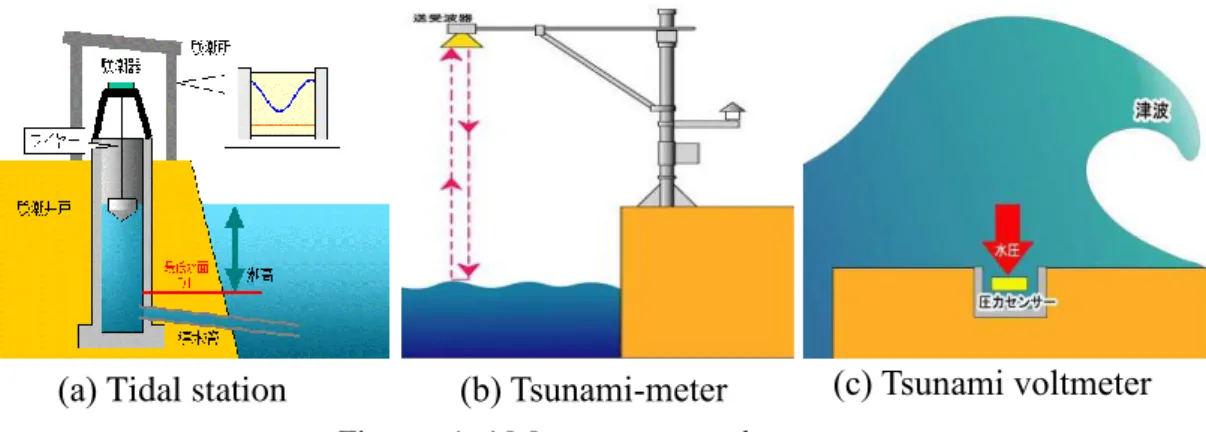
Due to the serious tsunami, the tsunami forecast research has made considerable progress. According to different criteria, the existing forecasting methods are divided into two categories [8]: the change of water pressure and the reflection of wave. Figure 1.4 shows some typical predictions based on changes of water pressure. In this category, predictive judgment is made by measuring changes of water pressure. This method of prediction is easy to set up and costs low relatively. However, when a real tsunami comes, pressure sensors are easily damaged and it is often difficult to predict the tsunami. Figure 1.4 lists three installations for tsunami measurements along the coast.
(a) A tide gauge (also known as a mareograph or, sea level recorder) is a device that used to measure changes of sea level relative to a vertical datum [9]. The sensor continuously records the height of the water level relative to the height reference surface near the geoid. Water enters the device through the bottom pipe. The device measures the height of water and sends the data to the computer.
Historical data is available for approximately 1,450 stations worldwide, of which about 950 have provided updates to global data centers since January 2010. Some places have recorded historical data for centuries, such as Amsterdam dating back to 1700. Used by satellite data, new modern tide gauge can often be improved.
Based on measuring the average sea level, tide gauge is used to measure tides and quantify the size of the tsunami. In this way, sea level slopes up to several 0.1m/1000km and more tsunamis can be detected. Tsunami can be detected when sea level starts to rise, although warnings from seismic activity may be more useful.
(b) The tsunami meter measures the height of sea level by transmitting the ultrasonic wave [10]. It is known as acoustic tsunami observation meter, which is usually placed above the water surface. First, the transmitter emits ultrasonic waves to the sea surface. Then, the height information of the water surface is measured by the time taken for transmission and reception of the ultrasonic waves. This method has the same advantages as the tide gauge station’s, such as simple structure, high precision and low cost. However, it also has the disadvantages of limited measurement range, easy damage and inability to be used for tsunami prediction.
7
(c) The Tsunami voltmeter consists of a pressure sensor. When the tsunami comes, the height of sea wave is measured by the voltmeter [10]. This system is simple and accurate. However, due to be installed on the coast, it cannot be used for tsunami prediction. In addition, the system is easy to be destroyed by the tsunami.
1.2.2 Measurement methods in long distance
Several common methods of measuring offshore altitude have been described above. Although these methods have different forms and principles, they all have the advantages of simple equipment and low cost. However, at the same time, there is a defect that the measurement range is small and it cannot be used for tsunami prediction. Therefore, if you want to predict the tsunami, you need to establish a method in the open-sea area or non-contact to measure tsunami.
Three types of long-range tsunami measurements are listed in Figure 1.5. Figure 1.5 (a) and Figure 1.5 (c) show the measurement system in the open-sea area. Figure 1.5 (b) shows a non-contact measurement.
(a) Tidal station (b) Tsunami-meter (c) Tsunami voltmeter
(a) GPS buoy (b) Tsunami radar (c) Observation networks
Figure 1.4 Measurements along coast
8
(a) The GPS Buoy (GB) system can be classified as an inverted long baseline (LBL) acoustic positioning device where the transducers is installed GPS-equipped sonobuoys that are either drifting or moored [11]. The GB can be used in conjunction with an active underwater equipment (such as a pinger-equipped torpedo) or with a passive acoustic source (such as inert bombs that strike the surface of the water). Time of arrival (TOA) techniques are commonly used to track or locate the sound source or impact event. Several GBs are often deployed in a given operating area; the total number is determined by the size of the test area and the accuracy of the desired result. You can use different GPS positioning methods to locate the array of GBs, with accuracies of the cm to meter level in real-time possibly.
(b) The tsunami radar can capture the tsunami in a distance of 30km from the sea surface and about 15 minutes before the tsunami arrives. Through transmitting and receiving radar waves, the observation frequency can reach once every two seconds [12-13]. However, it is difficult to measure the shape of the sea waves by this method. Especially for long-period and low-amplitude sea waves, the device is difficult to receive the returned waves after emitted by them. In addition, this device is also quite difficult to measure the distance of tsunami more than 30km.
(c) The Submarine Earthquake Tsunami Observing Network has set up a number of pressure sensor nodes on the seafloor [14]. The distance between node and node is about 20km and the coverage area is wide so that earthquakes and tsunamis can be observed as well as the tsunami arrival time can be predicted. However, the single node of the device has a limited measuring range and many disadvantages such as high installation cost, difficult maintenance, etc.
Although these two types of measurement methods do not have the ideal performance, the combination of the two type methods do some improvements. One of the famous combination methods is the DART (Deep-ocean Assessment and Report of Tsunami) [15]. Each DART station consists of a surface buoy and a seafloor bottom pressure recording (BPR) package that detects pressure changes caused by tsunamis. The surface buoy receives transmitted information from the BPR via an acoustic link and then transmits data to a satellite, which retransmits the data to ground stations for immediate dissemination to NOAA's Tsunami Warning Centers, NOAA's National Data Buoy Center, and NOAA’s pacific marine environmental laboratory (PMEL) [16]. The Iridium commercial satellite phone network is used for communication between 31 of the buoys.
When on-board software identifies a possible tsunami, the station will leave standard mode and start transmitting in event mode. In standard mode, the station reports water temperature and pressure (converted to sea level height) every 15 minutes. At the
9
beginning of the event mode, the buoys report the measurement every 15 seconds in several minutes.
The first generation DART I stations have one-way communication capabilities, and rely solely on software's ability to detect tsunamis to trigger event mode so that data transfers fast. In order to avoid false positives, the detection threshold is set relatively high, which may cause the low-amplitude tsunami not to trigger the station.
The second generation DART II is equipped with a two-way communication system that allows tsunami forecasters to change the station in event mode in anticipation of a tsunami’s arrival.
(https://nctr.pmel.noaa.gov/Dart/dart_ms1.html) Figure 1.6 Dart system
10
The above describes three tsunami technologies with large-distance measurement methods. Compared with near-distance tsunami measurements, long-distance measurements can detect from the coast to the ocean so that they can be applied to the tsunami prediction. Tsunami information can be obtained before the tsunami arrives. In particular, the GPS buoys and the DART, they are now relatively mature technologies and they are widely used in early warning systems for tsunamis. However, obviously, the existing problems are the high cost. They cannot monitor the large sea area. They can just detect the place where the buoy is near. There are still major problems to be solved.
For the task of monitoring tsunami, we need to obtain 3-D information such as the sea level height and the arrival time. Therefore, in view of the shortcomings of the existing sea level measurement methods and the advantages of the image measurement technology, this paper proposes a method of measuring the height of the sea level by using the 3-D image measurement technology to predict the tsunami.
11
1.3 3-D image measurement technology
The development of 3-D image measurement is rapid during recent years. They can be used widely for large range of wave heights measurement. 3-D image measurement methods also have the good performance in many fields. There are mainly three kinds of 3-D image measurement methods, which have been widely applied.
1.3.1 TOF method
The TOF (time of flight) method is similar to a radar that measures 3-D information by measuring the round time of the signal. System as shown in the Figure 1.7. For radar, the signal is microwave. For the TOF method, the signal is visible light. Figure 1.7 shows the structure diagram of the TOF method. The TOF method has the advantages of low cost. It is easy to use, and it has high precision. It has been widely applied in the fields of machine vision and 3-D scanning printing [17].
In TOF method, cameras, sensor and active light sources are necessary. It works by emitting the modulated light to the object and receiving the reflected light. It measures the circular time or phases shift between emission and reflection as well as converts it to distance. The light is usually near infrared. It is invisible to the human eye. The sensor should be designed to respond to the same spectrum.
Time-of-flight cameras for civil applications began to emerge around 2000,as the semiconductor processes became fast enough for such devices. The systems cover ranges of a few centimeters up to several kilometers. The distance resolution is about 1 cm. Compared to standard 2D video cameras, the lateral resolution of time-of-flight cameras is generally low and most commercially available devices at 320 × 240 pixels or less as of 2011. Compared to 3D laser scanning methods for capturing 3D images, TOF cameras operate very quickly, providing up to 160 images per second.
For the TOF sensor, an experiment was conducted to verify the measurement range. OPTEX's ZC-1050's TOF 3-D distance camera captures images of people at four different distances. For different distances, people's colors are different. The results show that the TOF sensor can only measure a distance of about 7 meters.
TOF sensors are not suitable for tsunami monitoring due to the measurement distance limitations. Just like radars, it consumes a lot of energy when the active measurement method is used for large area detection, which makes the cost too high to be realized.
12
1.3.2 Pattern projection method
This method is a 3-D scanning device for measuring the 3-D shape of an object using projected light patterns and a camera system. A typical system is shown in the Figure 1.8, including projector and regular camera [18]. First, the projector sends the pattern light to the object, and the camera takes image of the reflected projection. By using the correspondence between the projection pattern and the reflection pattern, 3-D space information can be extracted. A faster and more versatile method is the projection of patterns consisting of many stripes at once, or of arbitrary fringes, as this allows the acquisition of a multitude of samples simultaneously. Seen from different viewpoints, the pattern appears geometrically distorted due to the surface shape of the object.
Light source Object Sensor Computer Object Projector Reference plane Camera (http://www.idl.rie.shizuoka.ac.jp/study/project/tof/index_e.html) Figure 1.7 TOF system
13
Projection patterns can be divided into two types: binary patterns and non-binary patterns. Binary patterns include such as spot pattern, slit pattern or special coded pattern. Multi-projection is necessary and this procedure takes much time and slows down the whole measurement speed. Non-binary patterns include intensity gradient pattern, color modulation pattern. They simplify the multi-projecting into single or twice projecting, which are widely used nowadays.
1.3.3 Stereo vision method
Stereo vision is another popular 3-D measurement method which uses two separated cameras at the same scene or objects [19-20]. Figure 1.9 shows the basic components of the stereo vision method. The focal lengths of the two cameras are all f , the distance between the two cameras named as base line is b; and the corresponding projection points of target point P in the two images are represented as 𝑝1(𝑥1, 𝑦1) and 𝑝2(𝑥2, 𝑦2).
This method is based on a triangulation theory and recovers scene depth from the parallax of the images. The ideal structure is shown as Figure 1.10 which consists of two parallel camera images. 𝑂1 and 𝑂2 are the centers of camera images; the projection points of the target point P are 𝑝1(𝑥1, 𝑦1)and 𝑝2(𝑥2, 𝑦2)., equations (1.1) and (1.2) show how to calculate the distance Z by using the principle of similar triangles.
𝑓/𝑍𝑤 = 𝑥1/𝐿
(1.1) 𝑓/𝑍𝑤 = (−𝑥2)/𝑅 (1.2) 𝑏 = 𝐿 + 𝑅 (1.3) Z = 𝑏𝑓/(𝑥1 − 𝑥2 ) (1.4)
Figure 1.9 Stereo vision method
Target point: P Base line: b 𝑝1(𝑥1, 𝑦1) 𝑝2(𝑥2, 𝑦2) Y Z X 𝑂2 𝑂1
14
In order to find out the parallax, corresponding points matching is very important. Through stereo image rectification, images are projected onto a common plane which results in it that the corresponding points have the same row coordinates. This process helps reduce the 2-D stereo correspondence problem to a 1-D problem.
Target point: 𝑃(X𝑤, Y𝑤, Z𝑤)
𝑝1(𝑥1, 𝑦1)
𝑝2(𝑥2, 𝑦2)
Left image center b Right image center
L
f
𝑂1 𝑂2
15
1.4 The purpose of our research and structure of this paper
In the last section, we mention some progress achieved in short distance experiment. To realize the purpose of tsunami forecast finally, long distance measurement is a necessary process. This paper focuses on the long distance and we attempt to solve the problems occurring during the distance extension. The structure of this paper is as followed:
Chapter 1 explains the background of this paper and the existing forecast methods. In addition, it also proposes the conceive of forecast tsunami with 3-D image processing technology. This part introduces the system and finally gives the purpose as well as structure of this paper.
Chapter 2 introduces the calibration of binocular stereoscopic vision technology. First, we illustrate the theory of binocular stereoscopic vision.
Chapter 3 introduces the extraction methods of sea wave. First, we illustrate the difficulties in long distance sea wave extraction and then propose a partial analyze of pre-processing, double-threshold extraction method for different situations at long distance. This part explains the sea wave matching method. First, we introduce the difficulties of direct point matching and then explain the solution to this problem. Therefore, we propose the matching sea wave base on the feature matrix and show the results of this method.
In the chapter 4, we do some experiments. First, we introduce experimental conditions, and we propose to calculate the sea level through the average of many sea wave. Then, compare the calculated date with the data from the Meteorological Agency.
16
Chapter2 Calibration of long distance 3-D image
measurement system
Camera system calibration is an essential part in 3-D image measurement. The principle of ideal binocular stereo vision system is convenient. However, the two cameras in the measuring system are usually not parallel configurations in the actual measurement. In this case, the simple triangulation method cannot meet the requirements of calculation. We must configure the usual pin model of the binocular stereo vision.
Though many existing methods can calibrate cameras, but those methods are just effective to the close range, and they usually use a calibration target to calibrate the cameras. Since the distance of monitoring sea is very far, those methods are very difficult to apply the long-distance measurement, especially more than 20 kilometers. We construct a measurement system of long distance sea-level height for disaster prevention based on a 3-D image measurement technique. First, in order to monitor a wide range of the sea surface, this system utilizes the pan and tilt stages and angle sensors to rotate the cameras. In order to improve the accuracy of calibration, we use the standard scale pole to calibrate intrinsic and extrinsic parameters of cameras and angle sensors. In addition, all the equipment can be set in one place so it is convenient to maintain.
This chapter explains the principles of binocular stereo vision. Contrast with the exiting calibration, we propose the improved calibration method. Finally, experiments verify the calibration accuracy and it can meet the requirements of the system.
17
2.1 The theory of binocular stereoscopic vision
The camera model determines the geometric relationship of optical imaging of the camera. The simplest and most commonly used camera model is called the pinhole model, which is a linear model. The pinhole camera model is not a universal, wide-angle lens or some special lens, such as fish-eye lens, whose imaging rules are non-linear and cannot be solved with a pinhole model [21]. The camera used in this paper is the camera that meets the pinhole model.
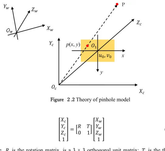
The imaging relationship of the pinhole model is shown in Figure 2.2. For any measurement point of space, its coordinates in the camera coordinate system can be represented 𝑃(𝑋𝑐, 𝑌𝑐, 𝑍𝑐). The position 𝑝(𝑥, 𝑦)of the image on the image plane satisfies the linear imaging rule, i.e. the projection position of the point P is the intersection of the line 𝑂𝑐𝑃 of optical center 𝑂𝑐and the point P of the camera to the plane of the image. This projection is also known as perspective projection.
To make it easier to understand the imaging process and geometry of points in the perspective projection model of the camera, it is necessary to understand the four coordinate systems associated with them, namely the image coordinate system, the image plane coordinate system [22], the camera coordinate system and the world coordinate system.
First, the image coordinate system is a coordinate system that describes the position of the pixel in the image. The digital image is stored in a computer in pixels. The computer divides the image into 𝑀 × 𝑁 small squares. each square is one pixel. As shown in Figure 2.1, the purple part of the image plane, the Cartesian coordinate system, is known as the image coordinate system. In general, the origin 𝑂0 of the image coordinate system is located in the upper left corner of the image. The coordinates (𝑢, 𝑣) in the coordinate system represent the number of rows and columns of a pixel in the digital image. However, only the image coordinate system cannot show the physical location of the pixel, so another coordinate system with a physical unit is needed. Such coordinate system is called the image plane coordinate system. In general, the origin 𝑂1of a plane-like coordinate system is defined at the intersection of the optical axis of the camera and the image plane, which is generally at the center of the image. The horizontal 𝑥 axis and the vertical 𝑦 axis are respectively parallel to the 𝑢 axis and the 𝑣 axis of the image coordinate system. We can assume that the origin of a plane coordinate system is expressed as 𝑢0, 𝑣0, and the physical dimensions of one pixel in the 𝑥 -axis and 𝑦 -axis directions are expressed as 𝑑𝑥 and 𝑑𝑦. Then, the coordinates of any pixel in the image in both coordinate systems are a conversion between (2.1) and (2.2).
18
𝑢 = 𝑥
𝑑𝑥+ 𝑢0 (2.1)
𝑣 = 𝑦
𝑑𝑦+ 𝑣0 (2.2)
(2.1) and (2.2) can be expressed as (2.3) in the form of homogeneous coordinates and matrix:
Figure 2.1 Images coordinate and the image plane coordinate
[ 𝑢 𝑣 1 ] = [ 1 𝑑𝑥 0 𝑢0 0 1 𝑑𝑦 𝑣0 0 0 1 ] [ 𝑥 𝑦 1 ] (2.3)
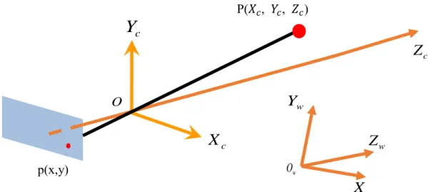
The other two coordinate systems are the camera coordinate system and the world coordinate system, which can be shown in Figure 2.2. The origin 𝑂𝑐 of the camera coordinate system is the lens center of the camera. The 𝑋𝑐 axis and 𝑌𝑐axis of the camera coordinate system are parallel to the x axis and 𝑦 axis of the image plane coordinate system, and the 𝑍𝑐 axis is perpendicular to the image plane, that is, the optical axis direction of the camera [23]. The intersection of the camera's optical axis and the image plane is the origin(𝑢0, 𝑣0) of the plane coordinate system, and the length of the connection 𝑂𝑐𝑂1 is the so-called focal length of the camera. The world coordinate system is a coordinate system used to describe the position of any object in the space including the camera. It is composed of 𝑋𝑤, 𝑌𝑤, 𝑍𝑤 axes. The conversion relation between the camera
u v x y 𝑂0 𝑂1
19
coordinate system and the world coordinate system can be expressed by a rotation matrix 𝑅 and a translation vector 𝑇 . Let the homogeneous coordinates of the measurement points 𝑃 in the world coordinate system be (𝑋𝑤, 𝑌𝑤, 𝑍𝑤, 1)𝑇 , and the homogeneous coordinate in the camera coordinate system is(𝑋𝑐, 𝑌𝑐, 𝑍𝑐, 1)𝑇 . There is a conversion between the two coordinates as shown in (2.4).
[ 𝑋𝑐 𝑌𝑐 𝑍𝑐 1 ] = [𝑅 𝑇 0 1] [ 𝑋𝑤 𝑌𝑤 𝑍𝑤 1 ] (2.4)
Where, 𝑅 is the rotation matrix, is a 3 × 3 orthogonal unit matrix; 𝑇 is the three-dimensional translation vector.
In general, the rotation matrix can be expressed by equation (2.5). Where, 𝛾, 𝛽, 𝛼 are the rotation angles based on the 𝑋-axis, 𝑌-axis and 𝑍-axis, the translation vector 𝑇 can be expressed by (2.6), 𝑡𝑋, 𝑡𝑌, 𝑡𝑍 is the parallel movement based on the 𝑋-axis, 𝑌-axis and 𝑍-axis. 𝑅 = [ 𝑐𝑜𝑠𝛼 −𝑠𝑖𝑛𝛼 0 𝑠𝑖𝑛𝛼 𝑐𝑜𝑠𝛼 0 0 0 1 ] [ 𝑐𝑜𝑠𝛽 0 𝑠𝑖𝑛𝛽 0 1 0 −𝑠𝑖𝑛𝛽 0 𝑐𝑜𝑠𝛽 ] [ 1 0 0 0 𝑐𝑜𝑠𝛾 −𝑠𝑖𝑛𝛾 0 𝑠𝑖𝑛𝛾 𝑐𝑜𝑠𝛾 ] = [ 𝑟1 𝑟2 𝑟3 𝑟4 𝑟5 𝑟6 𝑟7 𝑟8 𝑟9 ](2.5) x y P 𝑌𝑤 𝑍𝑤 𝑋𝑤 𝑌𝑐 𝑍𝑐 𝑋𝑐 𝑂𝑐 𝑂1 p(x, y) 𝑢0, 𝑣0
20 𝑇 = [ 𝑡𝑋 𝑡𝑦 𝑡𝑧 ] (2.6)
These are four coordinate systems associated with the camera perspective projection model [24]. After understanding the relationship between the various coordinate systems, you can understand and apply the camera imaging geometry better. The relationship between the equation (2.7) and the equation (2.8) can be obtained according to the proportional relation of its coordinates.
x =𝑓𝑋𝑐
𝑍𝑐 (2.7)
y =𝑓𝑌𝑐
𝑍𝑐 (2.8)
The relationship between the above perspective projection relationships (2.9) can be transformed by the homogeneous coordinate and matrix.
𝑍𝑐[ 𝑥 𝑦 1 ] = [ 𝑓 0 0 0 0 𝑓 0 0 0 0 1 0 ] [ 𝑋𝑐 𝑌𝑐 𝑍𝑐 1 ] (2.9)
The corresponding relation between the coordinates of the points in the world coordinate system and the coordinates of the projection points in the image coordinate system can be obtained in the equation (2.10).
𝑍𝑐[ 𝑢 𝑣 1 ] = [ 1 𝑑𝑥 0 𝑢0 0 1 𝑑𝑦 𝑣0 0 0 1 ] [ 𝑓 0 0 0 0 𝑓 0 0 0 0 1 0 ] [𝑅 𝑇 0 1] [ 𝑋𝑤 𝑌𝑤 𝑍𝑤 1 ] = [ 𝑓𝑥 0 𝑢0 0 0 𝑓𝑦 𝑣0 0 0 0 1 0 ] [𝑅 𝑇 0 1] [ 𝑋𝑤 𝑌𝑤 𝑍𝑤 1 ] = 𝑀1𝑀2[ 𝑋𝑤 𝑌𝑤 𝑍𝑤 1 ] = 𝑃𝑀 [ 𝑋𝑤 𝑌𝑤 𝑍𝑤 1 ] (2.10) In the equation 𝑓𝑥= 𝑓 𝑑𝑥 ,𝑓𝑦 = 𝑓
𝑑𝑦 , 𝑀1 is the internal parameter matrix of the
21
which is called the projection matrix.
Table 2.1 describes the specific meaning of each camera parameter. Among them, the internal parameter matrix 𝑀1 is only related to the internal structure of the camera, which
represents internal parameters including of camera focal length. The external parameters
𝑀2 are completely determined by the camera relative to the position of the world
coordinate system, called the external parameters of the camera. The process of solving these two parameters is called the calibration of the camera, and the calibration precision is related to the accuracy of the measurement results, which is a crucial link in the three-dimensional measurement [25-27].
This section firstly describes how to calculate the 3-D coordinates of an arbitrary point in a binocular stereo vision system under ideal conditions. The top view of the binocular stereo vision system is shown in Figure 2.3. There are two cameras on the left and right in the picture. The two cameras are identical. Light-colored oval-shaped part of the two cameras represents the lens and the focal length are 𝑓. Below the camera is the camera's imaging plane. The connection between the center of the left camera and the center of the lens of the right camera is called the baseline and the base line can be expressed in letters. If the optical axes of both cameras are strictly parallel and the camera's image plane is parallel to the baseline, such system is called the binocular vision system under ideal conditions.
Table 2.1 Camera parameters
Intrinsic parameters
Focus The vertical distance from the center of the camera lens to the image plane. The center of
image
The intersection of the optical axis with the image plane.
Pixel sizes The actual size of the pixel in the horizontal axis and the vertical axis. Distortion Distortion parameters generated by the
lens.
Extrinsic parameters
Rotation matrix Based on the orientation of the optical axis in three-dimensional space. Movement matrix Coordinate of camera’s optical center
22
The black object is the measured object in Figure 2.3, assuming that objects have a measurement point 𝑃. The left 𝑝1(𝑥1, 𝑦1)and right 𝑝2(𝑥2, 𝑦2) of two cameras shooting are left and right two projection point in the image coordinates. In addition, they are respectively according to the position of the two zero gap, which is as shown in Figure 2.4. The projection on the same point in the left view and projection on the right view on the same image contrast, the distance between them is the parallax [28]. According to the parallax point can be calculated relative to the distance measurement system (i.e. the depth information), the depth information of the measurement point 𝑃 and thus they can be used to get the measurement point which is relative to the corresponding three-dimensional coordinates measuring system. Then some simple derivation of the calculation process of the three-dimensional coordinate values is carried out.
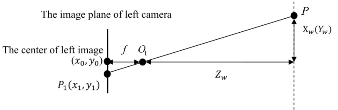
In order to obtain the three-dimensional coordinate information of the measuring point, the relative distance between the measuring point and the measurement system is firstly needed to measure the depth information of the measuring point based on the Z-axial direction of the measurement system [29]. Figure 1.10 is the calculation schematic diagram of the coordinates of the measuring points in the axial direction.
If you get a point in the direction of the axis, you can calculate the value of that point based on the other two dimensions. Figure 1.10 is the calculation principle of the coordinate values of the measuring points in the X-axis and Y-axis direction. As shown in Figure 2.4, it is in the direction of the horizontal axis (the X-axis) or on the vertical
Left camera Right camera
𝑝1(𝑥1, 𝑦1) b 𝑝2(𝑥2, 𝑦2)
f f
𝑝1 𝑝2
parallax
23
axis (Y-axis) direction. Once get the coordinates Z of the Z-axis direction, we just need the distance from the image point 𝑝1(𝑥1, 𝑦1) to horizontal distance and vertical distance of the center (𝑥0, 𝑦0) of the image, as shown in the equation (2.11-2.14). Similarly, the measurement point P is calculated according to the principle of similar triangles On the X-axis and Y-axis coordinate values.
Figure 2.4 The measurement theory of x and y axis 𝑥1 𝑓 = 𝑋 𝑍 (2.11) 𝑦1 𝑓 = 𝑌 𝑍 (2.12) 𝑋𝑤 = 𝑏𝑥1 𝑥2−𝑥1 (2.13) 𝑌𝑤 = 𝑏𝑦1 𝑥2−𝑥1 (2.14)
Finally, consolidating equations, the three-dimensional coordinate of the measuring point can be expressed by equation (2.15). Thus, the measured value of the point P calculated is the three-dimensional coordinate relative to the center of the left camera lens in the binocular stereo vision system.
[ 𝑋𝑤 𝑌𝑤 𝑍𝑤 ] = 𝑏 𝑥1−𝑥2[ 𝑥1 𝑦1 𝑓 ] (2.15)
The above pure ideal situation of the binocular stereo vision system computing flow. The center of left image
(𝑥0, 𝑦0)
X𝑤(𝑌𝑤)
The image plane of left camera
24
However, the reality of binocular vision system is not able to achieve such an ideal, which the light axis of the two cameras is strictly parallel and the imaging plane is parallel to the baseline [30]. At the time of actual configuration camera system, the placement of the cameras unavoidably some angles such as deviation, or already need a camera optical axis angle system to correspond to a specific measurement occasions. Under the condition of the wave height measurement, in order to realize the remote measurement at the same area of the measurement requirements, or achieve the purpose of extend measurement range, it is necessary to carry out the camera rotation. This configuration of binocular stereo vision system is shown in Figure 2.5, and there is an angle between the optical axis of the left camera and the optical axis of the right camera [31]. The three-dimensional measurement of the non-ideal conditions has a complete set of calculations. Its calculation method is based on the projection principle of space center point in the camera. The next section focuses on the relevant knowledge of camera perspective projection model.
Figure 2.5 The usual model of binocular stereo vision system
O1 O2 Z1 Z2 𝑝2(𝑥2, 𝑦2) 𝑃(X𝑤, Y𝑤, Z𝑤) 𝑝1(𝑥1, 𝑦1)
25
2.2 The existing calibration method
Direct linear transformation (DLT) is an algorithm which solves a set of variables from a set of similarity relations [32-34]. The direct linear transformation solution is a solution to establish a direct linear relationship between the coordinates of the coordinates (measured coordinates) and the coordinates of the corresponding object point shown as in Figure 2.6.
Figure 2.6 Calibration block of DLT method
There are many characteristics on the DLT. First, they don’t require the inner elements, without the orientation, which is suitable for a variety of non-measurement camera. Second, we do not need the initial value of the outer position, which is suitable for large angle close-up photogrammetry. Third, object space must be arranged a certain number of control points. Forth, in essence, it is a space rear intersection and front intersection solution.
In principle, the solution to the direct linear change is deduced from the collinearity equation. It is shown as in equation (2.16).
{ 𝑥 − 𝑥0 = −𝑓𝑎1(𝑋𝑤−𝑋𝑐)+𝑏1(𝑌𝑤−𝑌𝑐)+𝑐1(𝑍𝑤−𝑍𝑐) 𝑎3(𝑋𝑤−𝑋𝑐)+𝑏3(𝑌𝑤−𝑌𝑐)+𝑐3(𝑍𝑤−𝑍𝑐) 𝑦 − 𝑦0 = −𝑓 𝑎2(𝑋𝑤−𝑋𝑐)+𝑏2(𝑌𝑤−𝑌𝑐)+𝑐2(𝑍𝑤−𝑍𝑐) 𝑎3(𝑋𝑤−𝑋𝑐)+𝑏3(𝑌𝑤−𝑌𝑐)+𝑐3(𝑍𝑤−𝑍𝑐) (2.16)
26
Where (x, y) is the image point in the image plate coordinate system. (𝑥0, 𝑦0) is the center point of the image in the image plate coordinate system. (𝑋𝑤, 𝑌𝑤, 𝑍𝑤) is the coordinate of the object in the world coordinate system. (𝑋𝑐, 𝑌𝑐, 𝑍𝑐) is the coordinate of the object in the camera coordinate system. (𝑎𝑖, 𝑏𝑖, 𝑐𝑖) is the parameter of the rotation matrix.
Thus, the direct linear transformation has the remarkable characteristic that firstly the coordinates of the object space are directly transformed into the object space coordinates, so the initial values of the interior and exterior orientation elements are not needed. Secondly, the direct use of the original observation - image point coordinates, which can be effective system error compensation, especially for CCD camera calibration. Compared with the conventional camera calibration, there are two main aspects: the influence of the electrical error on the calibration; the algorithm requires fast real-time and it is stable and reliable.
Therefore, the CCD camera calibration often use the additional parameters of the direct linear transform method. When we consider the nonlinear distortion (radial optical distortion), the direct linear transformation method in the image space coordinates and the corresponding coordinates of the object are shown as follows:
{ 𝑥 − 𝑥0+ ∆𝑥 = −𝑓𝑎1(𝑋𝑤−𝑋𝑐)+𝑏1(𝑌𝑤−𝑌𝑐)+𝑐1(𝑍𝑤−𝑍𝑐) 𝑎3(𝑋𝑤−𝑋𝑐)+𝑏3(𝑌𝑤−𝑌𝑐)+𝑐3(𝑍𝑤−𝑍𝑐) 𝑦 − 𝑦0 + ∆𝑦 = −𝑓 𝑎2(𝑋𝑤−𝑋𝑐)+𝑏2(𝑌𝑤−𝑌𝑐)+𝑐2(𝑍𝑤−𝑍𝑐) 𝑎3(𝑋𝑤−𝑋𝑐)+𝑏3(𝑌𝑤−𝑌𝑐)+𝑐3(𝑍𝑤−𝑍𝑐) (2.17)
Where (∆𝑥, ∆𝑦) is correction number of the Linear error.
c
X
cZ
cY
wX
wZ
wY
w O O p(x,y) P(𝑋𝑐, 𝑌𝑐, 𝑍𝑐)Figure 2.7 Mapping relations between the images coordinate with the world coordinate
27
2.3 The improved calibration method
Though existing calibration method is effective for close range 3-D measurement, which is difficult for this technique. Those methods usually use a known plate to calibrate camera, but the distance is very long, it is difficult to make the plate. A calibration method to calibrate camera with long distance is proposed [35]. With this method, we calibrate the intrinsic parameters and extrinsic parameters of cameras, and calibrate the position relationship between the centers of pan and tilt head as well as camera center. Then, we can use the parameters of camera and the camera’s rotation angle to calculate the sea wave from long distance. The model is shown as in Figure 2.8.
To solve the problem of increasing deviation along with distance extension, a sequence of images are taken to calculate the parameters. We can use one known constraint to calculate parameters and obtain an optimal result.
By considering the leveling device of camera and fix the focal length of the camera, we simplify the process of calibration. Only the focal length of camera, rotation angle of Y-axis and baseline are considered in this method.
We use α, β, γ to represent the angle of X-axis, Y-axis, and Z-axis respectively. We suppose that γ equals to 0 and the original point is the center of the image. First, calculating the wave height roughly to test whether this method is feasible. The precise problem is considered later, and we can constrain the assumption while conducting experiment. We can just consider the degree of α . The degree of β doesn’t have influence on the parallax, and simplifies the perspective projection matrix as equation (2.18).
Figure 2.8 Calibration model Y Z Z2 Z1 Z O O α1 𝑓2 b 𝑓1 α2 β
28 𝑍𝑐 ∙ [ 𝑥 𝑦 1 ] = [ 𝑓 0 0 0 0 𝑓 0 0 0 0 1 0 ] ∙ [ 𝑐𝑜𝑠𝛼 0 0 1 −𝑠𝑖𝑛𝛼 𝑐𝑜𝑠𝛼𝑡𝑥− 𝑠𝑖𝑛𝛼𝑡𝑧 0 𝑡𝑦 𝑠𝑖𝑛𝛼 0 0 0 𝑐𝑜𝑠𝛼 𝑠𝑖𝑛𝛼𝑡𝑥+ 𝑐𝑜𝑠𝛼𝑡𝑧 0 1 ] ∙ [ 𝑋𝑤 𝑌𝑤 𝑍𝑤 1 ] (2.18) 𝑡𝑥 = 𝑑 (2.19) 𝑡𝑧= 0 (2.20) Where, 𝑍𝑐 is the distance from the world point to the parallax. The 𝑡𝑥, 𝑡𝑦, 𝑡𝑧 are the elements of the translation vector. The f is the local length of camera. [x, y, 1]T is the homogeneous coordinate of camera coordinate system, [𝑋𝑤, 𝑌𝑤, 𝑍𝑤, 1]T is the homogeneous coordinate of the world coordinate system, L is the distance between the center of pan and tilt head and the camera center. 𝛼 is the angle between the horizontal line of the center of pan and tilt head with the camera center. We can get equation (2.21) from the equation (2.18-20).
{
𝑓𝑐𝑜𝑠𝛼𝑋𝑤− 𝑓𝑠𝑖𝑛𝛼𝑍𝑤+ 𝑓(𝑐𝑜𝑠𝛼𝑡𝑥− 𝑠𝑖𝑛𝛼𝑡𝑧) = 𝑍𝑐𝑋 𝑓𝑌𝑤+ 𝑓𝑡𝑦 = 𝑍𝑐𝑌
𝑠𝑖𝑛𝛼𝑋𝑤+ 𝑐𝑜𝑠𝛼𝑍𝑤 + 𝑠𝑖𝑛𝛼𝑡𝑥+ 𝑐𝑜𝑠𝛼𝑡𝑧 = 𝑍𝑐
(2.21)
Simplify the equation (2.21) to equation (2.22)
(𝑓 − Xtanα)𝑋𝑤− (𝑓𝑡𝑎𝑛𝛼 + 𝑋)𝑍𝑤+ (𝑓 − 𝑋𝑡𝑎𝑛𝛼)𝑡𝑥− (𝑓𝑡𝑎𝑛𝛼 + 𝑋)𝑡𝑧 = 0 (2.22)
Set the original point of the left camera as the original point of the world coordinate system. The Z-axis of the world coordinate system is vertical to the base line, the X-axis of the world coordinate system is parallel to the base line, the Y-axis of the world coordinate system is parallel to the Y-axis of the camera coordinate system, we can obtain (2.23) from the equation (2.22).
{
𝑍𝑤 = 𝑏/(𝑡𝑎𝑛(𝛼1+ 𝑥1/𝑓) + 𝑡𝑎𝑛(𝛼2+ 𝑥2/𝑓)) 𝑋𝑤 = 𝑥1× 𝑍𝑤/(𝑓 × 𝑡𝑎𝑛(𝛼1+ 𝑥1/𝑓))
𝑌𝑤 = 𝑦1 × 𝑍𝑤/𝑓
29
Where, b is the length of base line, 𝑥1, 𝑥2 are the camera coordinate and 𝛼1, 𝛼2 are the degree with the Z-axis. Then the length of fence equation is followed.
𝐿 = √(𝑍𝑤1− 𝑍𝑤2)2+ (𝑋𝑤1− 𝑋𝑤2)2+ (𝑌𝑤1− 𝑌𝑤2)2 (2.24)
Where, L is the length of grid in every images.𝑋𝑤1, 𝑋𝑤2, 𝑌𝑤1, 𝑌𝑤2, 𝑍𝑤1,𝑍𝑤2 are the X-axis, Y-X-axis, and Z-axis world coordinate of the two different point in one image.
min = ∑𝑛𝑖=1(𝐿𝑖 − 𝐿) (2.25) Where, the known length of grid and this equation is optimized with the Levenberg-Marquardt method to obtain the unknown parameters. Equation (2.25) has four unknown parameters, b, 𝛼1, 𝛼2 and 𝑓.
30
2.4 Calibration experiments 2.4.1 Sea area in Shikashima
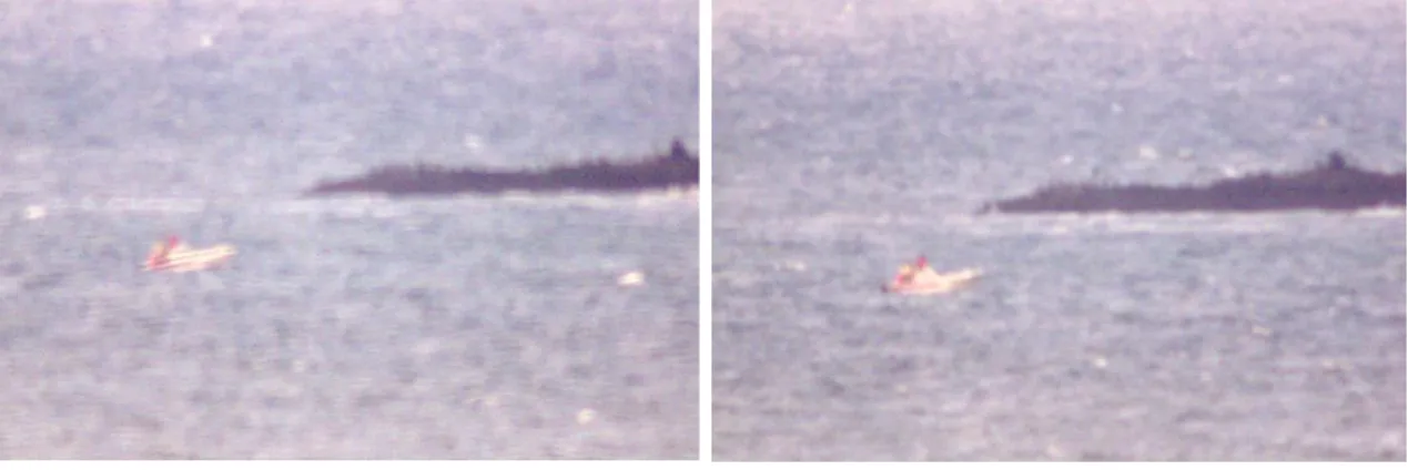
This experiment happened in Shikashima sea area as in Figure 2.9 shown. The distance is 5km. The accuracy of the wave height is affected by many factors. There are two main aspects, one is the measurement accuracy of the photographic system and the other is the correctness of the wave extraction. In order to verify the accuracy of the wave height measurement in the experiment, we use the ship marked with different colors to complete the experiment of measuring for the accuracy of the experimental camera.
Figure 2.9 The sea area in Shikashima
We put massive tags on the boat to obtain the length of boat from each image and four lengths of known boat can obtain the one set unknown parameters of the camera. We can obtain optimal set of parameter from massive solutions.
The ship's appearance is shown in Figure 2.10-12, with a length of 5.38 meters and the boat traveling on the sea. We take pictures of the ship in different locations. The camera take pictures at the same time and 10 sets of photos are taken for calibration.
Camera
31
Figure 2.11 Images at 12:30
Figure 2.12 Images at 13:15
Finally, followed by the coordinate of the boat, Table 2.2 shows the calibration results.
a. Left camera b. Right camera
a. Left camera b. Right camera
a. Left camera b. Right camera
32
Table 2.2 The result of calibration in Shikashima
Parameters Values
𝑓(pixel) 244620
𝛼1(°) -0.03
𝛼𝑧(°) -0.42
b(m) 40.91
Then we verify the calibration accuracy by measuring the length of the other photographs of the ship. The verification pictures are shown in Figure 2.13.
Figure 2.13 The images of calibration in Shikashima The results of measuring the length of the ship are summarized in Table 2.3
33
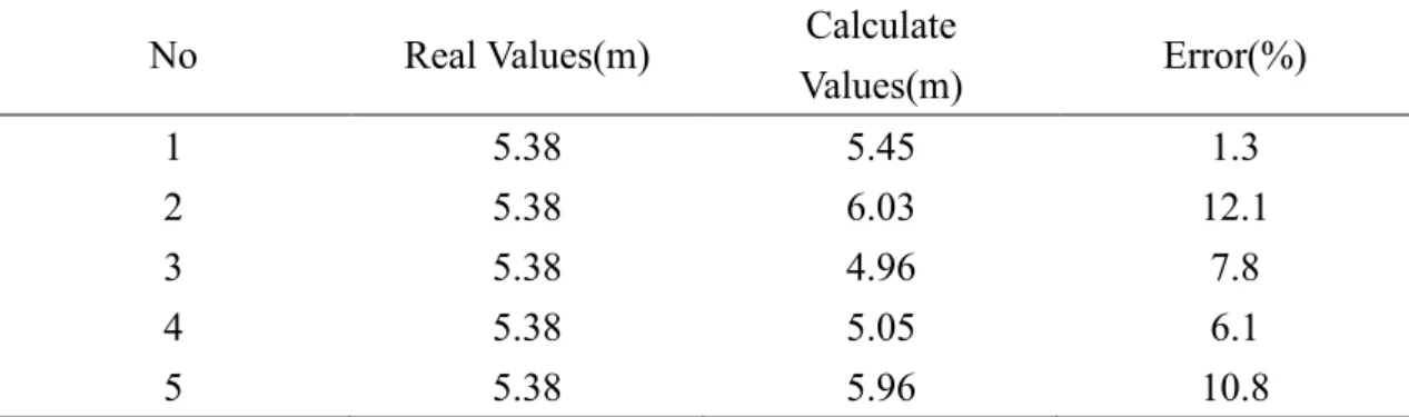
Table 2.3 The error of calibration in Shikashima
No Real Values(m) Calculate
Values(m) Error(%) 1 5.38 5.45 1.3 2 5.38 6.03 12.1 3 5.38 4.96 7.8 4 5.38 5.05 6.1 5 5.38 5.96 10.8
Table 2.3 is the result of distance between every person in the first calibration in which we can see that the max error is 12.1%, the min error is 1.3%, the average error is 7.6%, and the standard deviation is 3.79%.
2.4.2 Sea area in Shigu
The location of the experiment is on the shores of the Shigu as shown in Figure 2.14. The distance is about 5km. The calibration bar is shown in Figure 2.15. The shaft is red and white. The standard length of each small segment (red or white) is 0.5 m and the diameter is 0.65 cm. We choose a hollow plastic bar as a target and select the red and white boundary points on the central axis as feature points.
About 5Km
Camera Figure 2.14 Sea area in Shigu
34
In this experiment, everyone lifts the pole vertically in the designated place. The total number is four poles. In the first set of photos, the distance between the markers is 9m and 7m from left to right. In the second set of photos, the distances between the markers
Figure 2.16 Hollow plastic bar for calibration
a. Left camera (1) b. Right camera (1)
a. Left camera (2)
a. Left camera (3)
b. Right camera (2)
b. Right camera (3) Figure 2.15 Calibration image in Shigu
35
are 11m and 10m from left to right, and the distance between the two markers in the third group is 6m, which is shown in Figure 2.16.Finally, followed by the coordinate of the feature points, Table 2.4 shows the calibration result.
Table 2.4 The result of calibration in Shigu
Parameters Values
𝑓(pixel) 125620
𝛼1(°) 5
𝛼𝑧(°) 5.55
b(m) 29.95
Then we verify the calibration accuracy by measuring the length of the person. The
a. Left camera (1) b. Right camera (1)
a. Left camera (2)
a. Left camera (3)
b. Right camera (2)
b. Right camera (3) Figure 2.17 Verification images in Shigu
36
verification images are shown as in Figure 2.17.
The result of measuring the length between the bars is summarized in Table 2.5
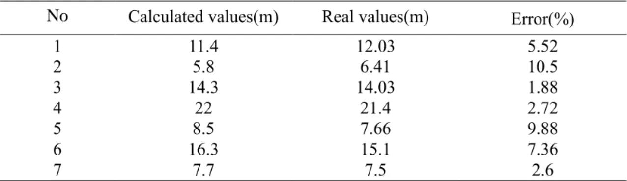
Table 2.5 The error of calibration in Shigu
No Calculated values(m) Real values(m) Error(%)
1 11.4 12.03 5.52 2 5.8 6.41 10.5 3 14.3 14.03 1.88 4 22 21.4 2.72 5 8.5 7.66 9.88 6 16.3 15.1 7.36 7 7.7 7.5 2.6
Table 2.5 is the result of distance between every person in the verification images in which we can see that the max error is 10.5%, the min error is 1.78%, the average error is 5.79%, and the standard deviation is 3.3%.
2.4.3 Sea area in Tsuyazaki
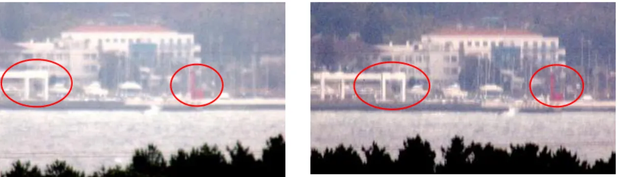
As the Figure 2.18 shown, the location of the experiment is on the shores of the Tsuyazaki. The distance is about 10km.
Figure 2.18 Sea area in Tsuyazaki
Tsuyazaki About 10Km
37
In this experiment, we firstly take a pair of images which include the red lighthouse and the iron shelves as shown in Figure 2.19.
Figure 2.19 Calibration Images in Tsuyazaki
Finally, followed by the coordinate of red lighthouse and iron shelves, Table 2.6 shows the calibration result.
Table 2.6 The result of calibration in Tsuyazaki
Parameters Values
𝑓(pixel) 244620
𝛼1(°) 20.42
𝛼𝑧(°) 20.22
b(m) 29.95
Then we verify the calibration accuracy by measuring the length of the other building. We extract five known lengths on the calibration object.
Table 2.7 The error of calibration in Tsuyazaki
No Calculated values(m) Real values(m) Error(%)
1 0.91 0.80 13.8
2 0.95 0.80 18.6
3 1.24 1.00 24
4 2.17 2.30 5.7
5 6.14 5.50 11.57
Table 2.7 is the result of the red lighthouse and iron shelves in the third calibration in which we can see that the max error is 24%, the min error is 5.7%, the average error is 14.36%, and the variance error is 3.7%.
38
2.5 Summary
Through the basic binocular stereo vision calibration described further, this section proposes an improved calibration method. Finally, the algorithm is verified by three experiments. In the three experiments, the error is the largest 12.8%, the smallest error is 1.06%, the standard deviation of error is 6.79. Through the experimental verification, the calibration method can meet the tsunami measurement and plays a key role in the future tsunami prediction.