鹿児島大学リポジトリ

Numerical Calculation of Tide in Kagoshima Bay

: Part 2. Two-dimensional Explicit Weighted

Residual Method

著者

KIKUKAWA Hiroyuki

journal or

publication title

鹿児島大学水産学部紀要=Memoirs of Faculty of

Fisheries Kagoshima University

volume

32

page range

29-48

別言語のタイトル

鹿児島湾の潮汐の数値計算 : 第2部 2次元の陽的重

みつき残差法

Mem. Fac. Fish., Kagoshima Univ.

Vol. 32 pp. 29-48 (1983)

Numerical Calculation of Tide in Kagoshima Bay

Part

2.

Two-dimensional

Explicit

Weighted

Residual Method

Hiroyuki Kikukawa

Abstract

The tidal residual flow in Kagoshima bay is evaluated by employing the two-dimensional explicit weighed residual method for space, which conserves the water mass, and the two-step

Lax-Wendroff method for time differentiation. Water surface elevation is given at the open

boundary and the non-slip boundary condition-is adopted at the coast. In order to obtain stable results, calculation is performed over five period.

The estimated tidal residual flow shows that there exists a large anti-clockwise vortex at

the center of the bay and that the water mass inflows from the east side and outflows from the west side of the mouth of the bay. In spite of the roughness of the division of the bay, the above two features of the results are similar to the observational results so far

performed.

1. Introduction

In the previous paper15, the tide in Kagoshima bay is calculated by making use of the primitive lumped mass marix method for two-dimensional horizontal space. The primitive lumped mass matrix technique is, however, known2) to be inadequate for the estimation of tidal residual flow because of the appearance of the energy loss in the

method, although the resulted tidal flow itself might be almost available3*.

In order to

improve this defect of the primitive lumped mass matrix method, Kawahara et al4)

proposed a selective lumping mass matrix method and calculated the tidal residual flow

of Osaka bay. In the selective lumping method, however, the time step has to be chosen to be smaller to avoid divergence in the calculation and then the calculation time needed becomes longer. Anyhow, the selective lumping technique is more artificial than

the primitive lumped mass matrix method.

For the purpose to decrease the energy loss in the calculation, we have proposed5* an

another explicit method named explicit weighted residual method or EWM for short. EWM is applied in this paper for the calculation of the tidal residual flow in Kagoshima

bay.

In the resulted tidal residual flow, the loss of water mass is 11.4 % at the open

Laboratory of Engineering Oceanography, Faculty of Fisheries, University of Kagoshima, Kagoshima 890

boundary and 3.8 %at the center of the bay, which may be admissible if the roughness

of the division of the bay is taken into account. There appears a large anti-clockwise

vortex at the center of the bay and the water mass inflows from the east side and

outflows from the west side of the mouth of the bay.

These two features agree

qualitatively to observations so far performed.

Some explanations of EWM are given in section 2 for the completeness of this paper.

In section 3 are presented the finite element formulations of Euler's equations of motion and equation of continuity, employing EWM for space and two-step Lax-Wendroff

scheme for time differentiation. The resulted tidal velocity, tidal mass transport, tidal

residual velocity, tidal residual mass transport etc. are shown in section 4. Section 5 is devoted to some discussions about the further improvement.

2. Explicit weighted residual method

Although EWM can be formulated also for the three dimensional and/or complex

element, only the two-dimensional simplex element is considered in this paper. In the

two-dimensional simplex element, any physical quantity q = q(xi, x2, t) is linearly

approximated as6)

q(xi, x2, t) = La(xi, x2)qa(t), (a = 1-3) (1) where qa denote the values of q at the ar-th vertex of the triangle element and La are

the area coordinates. In Eq. (1) the Einstein's summation convention is used for simplicity, i. e., the repeated Greek indices denote the summation over 1-3.

The weighting function q*(xi, x2) is taken to be the general linear function of coordinates (xi, x2) and then written as

q*(xi, x2) = Na(xi, x2)q2,

(a = 1-3)

(2)

where ql are arbitrary constants fixed at the #-th vertex of the triangle element and N

a(xi, x2) are also arbitrary linear functions of coordinates (xi, x2). The mass matrix M

is then defined by

Mafi = [NaLfidA,

(3)

where Q is the domain of the simplex element and dA denotes the area integral. For the finite element method to be explicit for space, the mass matrix has to be a diagonal matrix. In case of the Galerkin's method, however, the arbitrary linear functions Na

KlKUKAWA : Numerical Calculation of Tide 31

(4)

which is not a diagonal one. In Eq. (4), A denotes the area of the triangle element. In order to make the method explicit for space, the non-diagonal mass matrix of Eq. (4) is

artificially changed to the following diagonal matrix M in the lumped mass matrix

method

/ l 0 0 \

M=-y( 0 1 0 ,

(5)

\0 0 1/

General linear functions of coordinates Na can be written by using the area coordi nates La as

Na = a(a)La + b(a)Lfi + c(a)Lr, (a, 13, y cyclic) (6)

where a(a), b{a)y c(a) are arbitrary constants. The requirement of the diagonality of

the mass matrix, i. e. Man — 0 for a^ff, imposes the following two constraints among

the constants a(a), b(a), and c(a),

a(a)+2b(a)+c(a) = Q,

a{a)+b(a)+2c(a) = Q. (7)

Then b(a) and c(a) can be solved to be

b(a)= c(a)= ~\a{al

(8)

The weighting function, which gives the diagonal mass matrix, is uniquely determined

from Eqs. (2), (6) and (8) as

q*(xi, x2) = (3Li-L2-L3)^i* + (-Li + 3L2-L3)^2* + (-Li-L2 + 3L3)^3*,

(9)

where q$ are defined by a(a)qat/3. The diagonal mass matrix corresponding to the weighting function of Eq. (9) is written as

M=^-[ 0

0ail) 0

a(2) 0 1.

a{2) 00

(10)

Formulating the governing equations by the usual weighted residual method with the weighting function of Eq. (9) and considering qi{a = 1-N, TV is the total number of

the nodal points in the domain) as arbitrary constants, the method becomes explicit for

space.

For the purpose to make the method also explicit for time, the two-step

Lax-Wendroff time difference method is adopted in this paper. The details will be given in

the next section. In EWM, the equations to be overlapped are chosen to some combina

tions of those in the Galerkin's method so that they could be solved explicitly for space.

3. Finite element formulation by EWM

As the conservative form of equations are known5)to be more adequate for the

estimation of tidal residual flow than those of non-conservative form, the following

conservative forms of two-dimensional Eulef's equations of motion and equation of

continuity will be formulated by the weighted residual method,

dV_,du>_ ft

dt

dxi

u>

$>*;

(11) (12) (13)

KiKUKAWA : Numerical Calculation of Tide 33

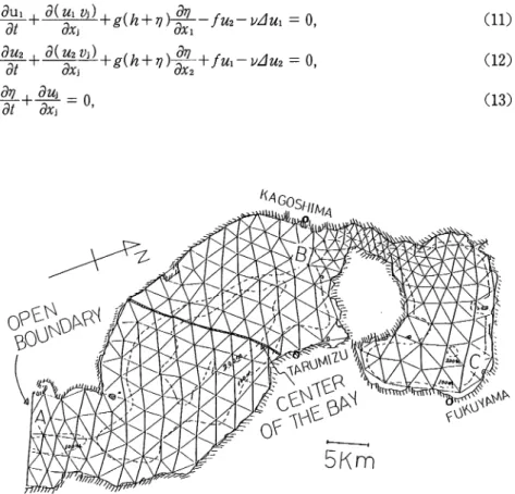
where Vi (i = 1, 2) denote the horizontal velocities, v the water surface elevation, h the depth of the bay, Ut = (h + v)vi, g the gravitational acceleration, / the Coriolis parame ter and v is the kinetic viscousity. In Eqs.(11)—(13), the repeated Latin indices denote the summation over 1 —2. In order to solve Eqs (11)—(13) in the domain of Kagoshima

bay, Kagoshima bay is preliminary divided into the two-dimensional simplex elements as shown in Fig. 1. Considering one of the elements in Fig. 1, the following variational functionals corresponding to Eqs. (11) —(13) are defined

+*£"&-*£(*£H

««

«-Mi+-&]"-

(16)

The integrals of the last terms of Eqs. (14) and (15) can be performed with the help of the Gauss' theorem. When all elements are summed up, these terms are cancelled by the neighbouring elements and in the case of the boundary elements, where the neigh bouring elements are absent, U\* and u* are taken to be zero at the boundary coast owing to the non-slip boundary condition adopted in this paper. Thus the last terms of Eqs. (14) and (15) can be cast away in the following.

In our case of EWM, the weighting functions ut, ut and y* take the form of Eq. (9).

Then approximating the physical quantities U\, u2 and rj as the linear functions of coordinates (see Eq. (1)), variational functionals of one element can be written as

dxfix = / Uia{Na[LpUifi + (LfiLr,xj + Lfi,xjLr)UifiVj7

_Jq

+gLf*L7tXXhfi + 7)ii)v7-fLfiU2ii} + vNa,xsLi3>XjUiii}dA, (17)

SXu2 = / U2a{Na[L0U2fi + (LfjLr,xj + Lp,xjLr)u2f}Vjr

+gL0L7,x2(hfi+ 7}0)7}r + fL0Uip] + vNa>xjLfi,XjU20}dA, (18)

where _ dUjg . _ drja Uja — ^. , V a • ~ dt ' j _ dLa »7 _ dNa

Laxj - dxj'

IVa-xl -

dxj'

Na = 3La-Lf-Lr (a, /?, r cyclic) = (V-'ULt,

(

3 _1 _1\

(!/-')= -1 3 \ - l -1 3/ (20) (21) (22)

In Eqs. (17) and (18), vja are taken to be uja/(ha+Va).

The method of weighted residuals requires SxUl, SxU2 and 8xv defined by

SxUl = 2

_elements

Sxilt

8xu2 =

_elements

2

8xeU2,

8xv =

_elements

2

Sxl

(23)

are vanished for any constants uta, uia and fjS for a = 1-Af, where Af is the total

number of the nodal points in the domain.

Instead, we could (i) first require 8xttu Sx

i2 and 8x* are vanished for any constants uta, uta and fji for a = 1-3 of one element

obtaining nine equations and then (ii) overlap the nine equations over all elements. The

number of the resulted equations is 3xjV.

Solving the 3x7V equations, the 3x7V

unknowns of U\a, u2a and Va for a = 1 - N can be resolved.

The nine equations obtained by the requirements of 8xux = SxeU2 = Sxl = 0 for any

constants uta, u2a and vi(a = 1—3) are

MapUi/} + KJapr( UipVjy + VjfiUi7) + gKip7(hp + Tjp)t}7

-/MapU2p+vRapUip = 0, (24)

MafiU2fi + Kifi7(u2fiVjY+VjfiU2r) + gKifir(hfi+ 7jfi)qr

+ fMapUip+vRapU2p = 0, (25)

MapVp+Ga/Ujp = 0, (26)

where

Map = [NaLpdA = (V~l)aP (LPLpdA = (V~l)aPMPp = -^Sap,

JQ JQ O

Kl» = fNaL,Lr*,dA = (V~l)„ [LtLfLr.xtdA = (V-1 W/&r,

JQ JQ

Rae = fnNa.xlLf,xldA = (V~x)„ fL,MLtMdA = (K"1 W?„,

JQ JQ

KlKUKAWA : Numerical Calculation of Tide

The integrals in Eq. (27) can be performed by using the integral formula7)

JULiLidA - (^Vc +2)/2A

i+b+c+2)r

Explicit integrations give the form of Eq. (4) for M and

^ap7 Ra b7 for a*ft 24 J_ 12b7 for a = 4A{babp + CaCp),

Gap —~~p~bp,

r2_{yjap — g}- -L where Cp,

2jc7 for a*t

1_ 12c7 for a = 0

ba = yp-yr, ca = x7—xp.{a, /?, r cyclic)

(28)

(29)

(30) 35

In Eq. (30), (xa, ya) is the coordinate of the a-th vertex of the triangle element. Eqs. (24) — (26) can be rewritten as

-yWia +(V'l)ap[Kip7(UipVj7+ VjpUi7) +gKp1p7(hp+Vp)T]7

—fMPp u2p + vRpp Uip] = 0,

^U2a +(V~l)ap[KPip7(u2pVj7 +VjpU27) +gKplp7(hp+7}p)7}7

+fMPpU\p+ vRPpu2p\ = 0,

-rTVa + ( V~l)apGJppUjp = 0,

(31)

(32) (33)

One of the commonly used explicit scheme for time differentiation is the two-step Lax-Wendroff method. The method implies

tM Q At '

(34) o r

qn+±= qn+±-Atqn,

where the upper suffices n, rc+y and »+l denote the time steps. Adopting the

two-step Lax-Wendroff method, it finally follows from Eqs. (31)-(33)

-J-UK* =-fufa+^^ftfa =-j-U?a ~4^{ V'^apF^p,

(36)

y-^a+2 =~fu2a-^f( V-1 )apFS2p,

(37)

-j-vS^ =-y*"--T"( V-l)a,Ff»

(38)

"juU1 =^m?«+J/-yitf«+i =-y«fa-4/( V-l)apF2$,

(39)

-yw?«+I ="jula-Ati V-l)apF£2+pi

(40)

-y^+1 ="jVa-Ati V-l)apF?P+i

(41)

with

FUlP = Kpip7(uipVj7 + VjpUi7)+gKp1p7(hp + 7}p)i?7

-fMppu2p + vRppU\p, (42)

Fu2P = Kpip7(u2pVj7 + Vjpu27)+gKp2p7(hp + 7ip)7}7

+ fMPpUip + i>Rppu2p, (43)

Fr,P = GppUjp. (44)

Summing up Eqs. (36) - (38) over all elements and solving the resulted 3x N equations,

the 3x AT unknowns of uTa^, u&* and vS^ (a = 1-AO can be resolved from the 3x

N known values of u?a, u?a and ^ (a = 1-AO. Next, summing up Eqs. (39)-(41)over

all elements and solving the resulted 3xN equations, the 3xN unknowns of u?Z\ utt1

and vS+l (a = 1 - N) can be resolved from 6x A known values of u?a, ula, vl vRi%,

u2a^ and 7ja+ 2" (a = 1-A).

Then we can proceed to the next step.

4. Results

The division of Kagoshima bay into two-dimensional simplex elements is given in Fig.

1, which is the same as was used in the previous paper1*. At first some discussions about the stability of the calculation are inevitable. Gray and Lynch8) investigated the stability conditions for the one-dimensional tidal flow equations without nonlinear

convective terms and found that the time step At is limited by

/}t^UxTLi

(45)

4 v

1 Armin

KlKUKAWA : Numerical Calculation of Tide 37

in the case of the usual Galerkin's finite element method with the two-step Lax-Wendroff time differentiation scheme. Nishi-Sakurajima channel gives the minimum

value of Ax to be Axmm ^ 103 m. Then taking into account the experimental value of the kinetic viscousity v being 105-107 (cm2/sec), Eq. (46) is found to give a more severe restriction for the time step than Eq. (45). If the depth of Nishi-Sakurajima channel is

taken to be 40 m, the upper boundfor the time step is estimated from Eq. (46) to be about

29 seconds. No other places give more severe restriction to At than 29 seconds.

Actually, however, the unstable divergenceoccurs even if At is chosen to be 15 seconds.

The more rigorous restiction than Eq. (46) might be caused by the two-dimensionality of our problem and the inclusion of the nonlinear convective terms. Calculation is performed by taking 10 seconds for the time step, which gives stable results.

The non-slip boundary condition is adopted at the coast and at the entrance of Kagoshima bay, the harmonic oscillation of water elevation is given with amplitude 1 m and period 12.5 hours. Owing to the oscillatory boundary condition at the open bounda

ry, the water mass transport integrated over one tidal period (WMT) at any cross

section of the bay must be vanished, or in other words, the inflow part of WMT

(WMTIN) and that of outflow part (WMTOUT) have to be equal to each other.

Calculation is performed over five periods. The time variations of WMTIN and

WMTOUT at the open boundary and at the center of the bay shown in Fig. 1 are

represented in Fig. 2. At the fifth period,

Fig. 2

v000m3/sec)

50r 5r

30- 3

OPEN BOUNDARY

CENTER OF THE

.

.

BAY

x *. #. *

20

10

-

2

-2

3

U

PERIOD

WMTIN (• ) and WMTOUT (x ) at the open boundary (dashed line) and at the center of the bay (solid line) of Kagoshima bay with respect to period

WMTIN = 3.768xi03m3/ sec,

WMTOUT

WMTIN 0.886,

at the open boundary and

WMTIN = 4.933xi02m3/sec, WMTOUT WMTIN = 0.962, WMTOUT = 3.338Xl03m3/sec, (47) WMTOUT = 4.746 Xl02m3/sec, (48)

at the center of the bay. The 3.8% loss of water mass at the center of the bay could be admitted from the point of relatively rough division of the bay. The 11.4% loss of

water mass at the open boundary could be improved if the finer divisions of there and

of the Nishi-Sakurajima channel are employed. In fact, in the case of Shibushi bay 5) where nine nodal points exist at the open boundary, the loss of water mass is estimated

to be only 2.8%. In the Nishi-Sakurajima channel, only two nodal points are there and

WMTIN is much larger than WMTOUT, which might be also one of the causes of the loss of water mass at the open boundary.

The resulted tidal residual mass transport at fifth period is shown in Fig. 3. As can

be seen from the figure, there exists a large anti-clockwise vortex at the center of the bay and water mass inflows from the east side and outflows from the west side of the

mouth of the bay. These two features of the tidal residual mass transport are similar to the observational results so far performed. At Nishi-Sakurajima channel, water

mass looks like to inflow from the west side and to outflow from the east side of the

Fig. 3 The distribution of the tidal residual mass transport in Kagoshima bay

KlKUKAWA : Numerical Calculation of Tide 39

channel. The water mass transport of there, however, is not well conserved and

further investigation by a finer division of the channel must be inevitable. The

distribution of the tidal residual velocity is given in Fig. 4, the shape of which is very

similar to Fig.3 except the relative smallness of the strength of the anti-clockwise

vortex. The tidal residual mass transport consists of that proportional to the tidal

Fig. 4 The distribution of the tidal residual velocity in Kagoshima bay calculated by EWM.

Fig. 5 The distribution of (tidal residual mass transport-tidal residual velocity x depth) in Kagoshima bay calculated by EWM.

residual velocity and of the Stokes mass transport. The Stokes mass transport vanishes if the tidal wave is the standing wave. (Tidal residual mass transport-tidal residual velocity x depth) are depicted in Fig. 5, the main part of which is the Stokes

mass transport. The conspicouous differences of this figure from Figs. 3 and 4 are (i)

(a)

(b)

Fig. 6 Tidal water mass transport distributions at / = 6.25 hour (6a) and at t = 12.5 hour (6b) in Kagoshima bay calculated by EWM.

KlKUKAWA : Numerical Calculation of Tide

(a)

Fig. 7 Tidal velocity distributions at / = 6.25 hour (7a) and at / = 12.5 hour (7b) in

Kagoshima bay calculated by EWM.

41

the water mass inflows from the west side and outflows from the east side of the mouth of the bay and (ii) at the offshore of Tarumizu-city the water mass flows to the southern direction. The distributions of the tidal water mass transport (velocity) at t

(m)

10 -^^~~ """V^*. **"

0.5

/ / / / / / X'» N X** s \

6 / /

\ r N 0 / \ i i i I 1 1 /' /I 1 1

1

1

l \

V\1

2

3

A 5 / / I

8

9

10 11 12 0.5 \ \ — \ ^ X \ A' / / / /

HOUR

X. V

yy'/

1.0 y\'"" s

Fig. 8

Time variations ofwater surface elevations at points A(solid lime), B(dotted

lime) and C (dashed lime) shown inFig. 1 calculated by EWM.

In Fig. 8 is given the time variation of the water surface elevation of the fifth period at the open boundary (A), at off Kagoshima city (B) and at off Fukuyama city (C),

where the points A, B and C are shown in Fig. 1. The phase delay of point B (C) with respect to the point A is seen to be about 6 minutes (32 minutes), which was about 20

minutes (90 minutes) in case of the primitive lumped mass matrix method. Although

the phase delay seems to be still larger than the observational one, the contradiction

between them is much improved in the EWM from the lumped mass matrix case. The

amplitude of water surface elevation at the point B (C) is about 5.8% (9.2% ) larger than that at the point A, which was about 4.0% (-7.5% ) in case of the primitive

lumped mass matrix method0.

5. Discussions about the further improvement

(i) The finer division of the bay is inevitable to improve the water mass conservation, especially at the Nishi-Sakurajima channel and at the open bounndary. The contradic tion between the calculated phase delay and the observational one would be decreased also by the finer division.

(ii) An another improvement could be done by adding the outer part of bay into the

calculational area. This addition might be especially important to investigate the pattern of tidal residual flow at the mouth of the bay.

(iii) The other boundary conditions, slip boundary condition at the coast, velocity or

KlKUKAWA : Numerical Calculation of Tide 43

also to examine whether .the results owe to the boundary conditions abruptly or not.

(iv) In order to compare the calculated results with the observational ones, it must be inevitable to investigate the influences of winds, to give a more realistic water surface elevation at the open boundary, to extend the method to the three dimensional case and

to take into account the influences of density, etc..

Acknowledgements

The author is very grateful to Dr. H. Ichikawa for many instructions about the

oceanography. He also owes to Mr. I. Seo, Mr. H. Nishi, Mr. A. Soejima and Mr. H.

Uchiyama for writing the figures by the X-Y plotter and the estimations of the conserva tion of water mass transport. Calculation is performed by FACOM M-200 in Kyushu

Univ..

Appendix Comparison between EWM and primitive lumped mass matrix method and

between conservative form and non-conservative form

For completeness of this paper, EWM is briefly compared with the primitive lumped

/ / / / / / / / / / / / / / / / / / / / / / / / / / / / / / / / / / / // / / LL• 2 // O •to / / <l UJ / / / / Q l Z) Z LL] .UJ • x / / / / / o U / CC\\ /

z h A / V

UJl\_~/\

/\

/

hu^d-

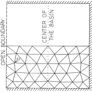
/ s LJ l^^ 1 A S s y y ' / / / / / / / / / / / / / / / / / // / / / / / / /? / / / / / / / / 's

Fig. 9 Model basin and its division into two dimensional simplex elements. Because

of the symmetry of the basin, calculations are performed only in the lower half

mass matrix method and conservative form of equations with the non-conservative

ones. Comparison is made for the rectangular model basin shown in Fig. 9 with

constant depth. The non-dimensional governing equations without Coriolis force are

given by

&»>&*&-**-*.

CA-D

-|+^-[(l+t,toJ =0,

(A-2)

for non-conservative forms and

M-+JimA+m +e,>g.-EjUl =l>.

(A-3)

$+-&-*

(A-4)

for conservative forms. All quantities in Eqs. (A-l)~(A-4) are non-dimensional ones and

(A-5)

(A-6)

where a is the amplitude of the tide at the open boundary, T the period of the tide and

/ denotes representative length of the basin. For EWM, the equations to be summed up

over all elements are written in analogy with Eqs. (36)—(41) as

TqS+* =TQS~^f{ v~l )apF*p>

(A ~7)

-fqS+1 =-fqS-At( V-^apF&i

(A -8)

where q represents vt (i = 1~~2) and v for non-conservative case and Ui (i = 1~2) and

V for conservative case. For the lumped mass matrix method, the equations correspond

ing to Eqs. (A-7) and (A-8) are

-fqS+^ =MapqS-^-Fqna,

(A -9)

-ytfH =MapqS-AtFZa+i

(A -10)

where Map is that defined in Eq. (4). In Eqs. (A-7) ~~ (A-10), Fq are written as

Fvta = £Kip7Vjpvi7+AGapyp+ERapVip, (A -11) Fna = Kifir[Vjfi(l + £y7)+(l + £Vfi)Vjrl (A "12)

p - a x - -gT2h

F-vT

£- h'

A-

I2 '

KlKUKAWA : Numerical Calculation of Tide 45

for non-conservative form and

FUia = eKip7(UipVj7+ VjpUi7) + AKip7(l + £7}p)7}7 + ERapUip, (A -13)

Fva = GipUjp, (A -14)

for conservative form.

Non-dimensional parameters are chosen to be £ = 0.05, A = 5080 and E = 0.01 corre

sponding to Yanagi's indoor experiments9* of a = 0.5 (cm), h = 10 (cm), T = 360 (sec), / = 500 (cm) and v —7 (cm2/sec), which is the fundamental experiment for tidal and

tidal residual flows. Water surface elevation is given at the open boundary and non-slip

boundary condition is adopted at the coast. Time step At is chosen to be 1/3600 taking

into account the stability condition of Ref. 8. For EWM calculations are performed over 9 periods in order to get stable results and for primitive lumped mass matrix method only two periods calculations are satisfactory. In fact in the latter case, the results in the third period are equal to those at the second period up to five figures.

The resulted tidal residual mass transports are given in Figs. 10 —13 and WMTIN and WMTOUT together with the loss of water mass at the open boundary and at the center

of the basin are listed in Table 1. From Figs. 10 —13 and Table 1, it can be seen that (i)

the water mass is lost completely in the primitive lumped mass matrix case independent

of the forms of the employed equations and (ii) in the EWM, the conservative forms of

governing equations looks like to be more adequate than the non-conservative ones to estimate the tidal residual flow.

0.002

Fig. 10 The distribution of the tidal residual mass transport in a model basin

calculated by the primitive lumped mass matrix method with non-conservative form of equations.

/

X

/

/

0.02

Fig. 11 The distribution of the tidal residual mass transport in a model basin calculated by EWM with non-conservative form of equations.

0.002

Fig. 12 The distribution of the tidal residual mass transport in a model basin calculated by the primitive lumped mass matrix method with conservative

KlKUKAWA : Numerical Calculation of Tide 47

X

/

/

/

/

0.02

Fig. 13 The distribution of the tidal mass transport in a model basin calculated by

EWM with conservative form of equations.

Table 1. Balances of water mass tranport in a model basin calculated by EWM and the primitive lumped mass matrix method with conservative and

non-conservative forms of equations.

Lumped mass matrix method EWM (ninth period) non -conservative form conservative form non-conservative form conservative form o WMTIN 0.277XKT2 0.462X10"3 0.861 X10"2 1.126X10"2 3 WMTOUT 0 0.018X10"3 0.695X10"2 0.994X10"2 c r o c 3 0-p WMTOUT WMTIN 0 0.039 0.807 0.883 -1 ••< Loss of water m a s s 100% 96.1% 19.3% 11.7% o WMTIN 0.948X10"3 0.105X10'2 0.795X10"2 0.805 X10"2 3 CO WMTOUT 0.019X10"3 0 0.760X10"2 0.799X10'2 o WMTOUT WMTIN 0.020 0 0.956 0.992 c r 5' Loss of water m a s s 98.0% 100% 4.4% 0.8%

Refferences

1) H. KIKUKAWA and S. KURIYAMA : Numerical calculation of tide in Kagoshima bay Part

1. Two dimensional explicit method, Mem. Fac. Fish., Kagoshima Univ. 29 (1980) 169-177.

2) mtim%, mmmik, 'M*H|?, JIISBA : &&M-j£|®Lax-Wendroff ftoaiB^S^SA^OJcE

ffl, I2 0lii(otifl^tf->y^^nim (19 8 0) 105-110.

3) M. KAWAHARA, N. TAKEUCHI and T. YOSHIDA : Two step explicit finite element method for tsunami wave propagation analysis, Int. J. Numer. Meth. Eng., 12 (1978) 331-351.

4) M. KAWAHARA, H. HIRANO, T.TSUBOTA and K. INAGAKI: Selective lumping finite

element method for shallow water flow, Int. J. Numer. Meth. Fluid, 2 (1982) 89-112. 5) H. KIKUKAWA and H. ICHIKAWA: An improved explicit finite element method for tidal

flow, Int. J. Numer. Meth. Eng., to be published.

6) 0. C. ZIENKIEWICZ (1977): The Finite Element Method, 3-rd Eddition, McGrow-Hill.

7) M. A. E. EISENBERG and MALVERN : On the finite element integration in natural coordi

nates, Int. J. Numer. Meth. Eng., 7 (1973) 574-575.

8) W. G. GRAY and D. R. LYNCH: Time-stepping schemes for finite element tidal model

computations, Adv. Water Resour., 1 (1977) 83-95.

9) Y. YANAGI: Fundamental study on the tidal residual circulation-I, J. Oceanogr. Soc. Japan 32(1976)199-208,: Fundamental study on the tidal residual circulation-I I,J. Oceanogr. Soc.