Absolute Measurements of PhotoluminescenceQuantum Yields of Organic Compounds Using anIntegrating Sphere

Absolute Measurements of Photoluminescence

Quantum Yields of Organic Compounds Using an

Integrating Sphere

Atsushi KOBAYASHI

Gunma University

Acknowledgment

I would like to express my sincerest gratitude to Professor Seiji Tobita, for his insight direction, valuable suggestions and discussions throughout this study. I wish to thank Associate Professor Minoru Yamaji for his experimental guidance and comments. I also wish to thank Assistant Professor. Toshitada Yoshihara for his valuable advice and discussions. I would like to express my thanks to Dr. Kengo Suzuki for his valuable suggestions and comments.

I am also sincerely grateful to Professor Hiroshi Hiratsuka, Professor Takeshi Yamanobe, Professor Masafumi Unno, and Professor Yosuke Nakamura for their valuable comments and kind advises on this thesis.

I would like to express my graduate to Dr. Kazuyuki Takehira for his valuable discussions, encouragement and experimental guidance. I also would like to express thanks to Mr. Hijiri Nakajima for his advice, encouragement and experimental guidance. I am grateful to Dr. Satoru Shiobara and Dr. Hirofumi Shimada for their valuable advice and comments. I show my gratitude to Dr. Juro Oshima and Dr. Shigeo Kaneko for their encouragement. I show my thanks to Ms. Tokiko Murase for her assistance. I acknowledgment to Mr. Tokio Takeshita and all laboratory members for their valuable suggestions and assistance to complete this work.

Finally, I would like to express my deep gratitude to my family for their supports me in every respect.

Contents

Chapter I

General Introduction

I-1 Luminescence quantum yield

... 2

I-2 Absolute method

... 6

I-2-1 Vavilov method ... 6

I-2-2 Weber and Teale method... 13

I-2-3 Calorimetric method ... 15

I-3 Relative method

... 18

I-4 The purpose of this study

... 21

References

... 22

Chapter II

Experimental

II-1 Absolute measurements of luminescence quantum yields using

an integrating sphere

... 24

II-2 Absorption and emission spectra

... 29

II-3 Fluorescence lifetime

... 29

II-5 Photoacoustic measurments

... 35

Appendix

... 40

References

... 44

Chapter III

Absolute Measurements of Luminescence Quantum Yield of

solutions at Room Temperature

III-1 Introduction

... 46

III-2 Materials

... 47

III-3 Results and Discussion

... 50

III-3-1 Spectral sensitivity of instrument ... 50

III-3-2 Effects of reabsorption and reemition ... 55

III-3-3 Fluorescence quantum yields of standard solutions... 60

III-3-4 Fluorescence quantum yield of quinine bisulfate ... 62

III-3-5 Fluorescence quantum yield of 9,10-diphenylanthracene ... 71

III-4 Conclusions

... 80

References

... 81

IV-1 Introduction

... 85

IV-2 Experimental

... 85

IV-3 Results and Discussion

... 89 IV-3-1 Luminescence quantum yields of 9,10-diphenylanthracene and

benzophenone at 77K ... 89 IV-3-2 Fluorescence and phosphorescence quantum yields of naphthalene

and 1-halonaphthalenes at 77K ... 91 IV-3-3 Phosphorescence quantum yields of benzophenone and

4-halobenzophenones at 77K ... 103

IV-4 Conclusions

... 107

References

... 108

Chapter V

Chapter I

I-1 Luminescence quantum yield

The relaxation processes of an excited molecule consist of radiative and nonradiative processes. “Fluorescence” is defined as the radiative transitions occurring without change in the spin multiplicity in a molecule, and “phosphorescence” is defined as those with change in the spin multiplicity. In a similar manner, “internal conversion” is defined as nonradiative transitions without change in the spin state, and “intersystem crossing” is defined as those with change in the spin state. Figure I-1 illustrates various rate processes included in the relaxation processes of an excited molecule.

There are four characteristics that can be associated with a molecular luminescence: (a) energy, (b) quantum yield, (c) lifetime, and (d) polarization. From absorption and/or emission wavelength, one can construct an energy state diagram of the molecule. The quantum yield and lifetime are essential photophysical quantities to determine the rate constants for the radiative and nonradiative processes, i.e. kf, kp, kic, kisc, and kisc’.

Polarization of absorption and emission is related to the electronic structure of the excited state involved in the transitions. It has long been recognized that among the photophysical quantities (a)-(d) the quantum yield is one of the most difficult quantities to determine the accurate value [1,2].

The photoluminescence quantum yield is defined as the ratio of the number of emitted photons to that of absorbed photons as follows.

The fluorescence quantum yield:

1 0 f 0 1 f to exciting in absorbed quanta of number emitted, quanta of number S S h S S → +

ν

= Φ (I-1)

The phosphorescence quantum yield:

1 0 p 0 1 p to exciting in absorbed quanta of number emitted, quanta of number S S h S T → +

ν

= Φ (I-2)

For the Φf, Φp, the quantum yield of S1→S0 internal conversion (Φic), and the quantum

yield of S1→T1 intersystem crossing (Φisc), the following relations are derived. f f f =k

τ

Φ (I-3) f ic ic =k

τ

Φ (I-4) f isc isc =k

τ

Φ (I-5) isc p p p = Φ Φ kτ (I-6)

where

τ

f and

τ

p are the fluorescence and phosphorescence lifetimes. Based the

measurements of Φf, Φic, Φisc, Φp,

τ

f and

τ

p, the rate constants kf, kic, kisc, kp can be

evaluated, and then kisc’ is given by

p p isc k

k '=τ−1− (I-7)

The luminescence quantum yield measured for a molecule in solution varies depending on the experimental conditions, including the kind of solvent, the concentrations of sample molecules and dissolved oxygen in the solution, temperature, and excitation wavelength. When the physical conditions are fully specified, the absolute quantum yield can, in principle, be precisely determined. However, even if these parameters are specified, a number of pitfalls exist, which must be considered explicitly to determine reliable quantum yields. These include polarization effects, refractive index effects, reabsorption/reemission effects, internal reflection effects, and the spectral sensitivity of the detection system [3,4].

Representative methods for the determination of luminescence quantum yields are listed in Table I-1. The principle of these methods is briefly reviewed in the following sections.

VR

VR

VR

VR

VR

IC

ISC

ISC

IC

Fluorescence

Phosphorescence

S

₀

S

₁

S

₂

T

₁

T

₂

h

ν

IC : Internal conversion

VR : Vibrational relaxation

ISC : Intersystem crossing

Figure I-1 Relaxation processes of organic compound

(k

_ic

)

(k

_isc

)

(k

_isc

’)

Method

I. Absolute Method Vavilov method (using magnesium oxide as a standard)

Weber and Teale method (using solution scatterer as a standard)

Calorimetric method Integrating Sphere method II. Relative Method Optically Dense method

Optically Dilute method

I-2 Absolute method I-2-1 Vavilov method

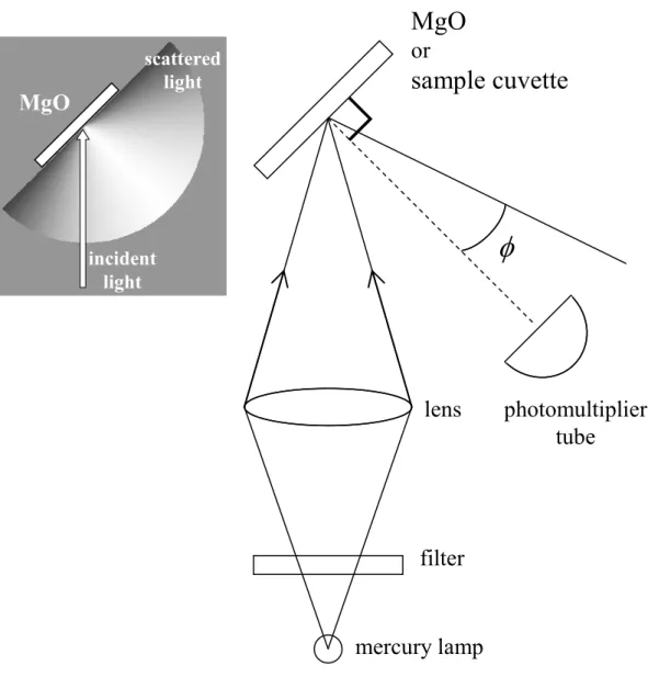
Over the past several decades, considerable efforts have been made to develop reliable methods for determining luminescence quantum yield [3,4]. As summarized in Table I-1, they can be classified into absolute (or primary) methods and relative (or secondary) methods. The first reliable absolute method was developed by Vavilov [5]. In the Vavilov method, a solid scatterer (magnesium oxide) is used to calibrate the detector/excitation system absolutely. The detector first monitors the sample luminescence generated by total absorption of the excitation light focused to a point in the cell. The detector then records the light that is diffusely scattered from the magnesium oxide surface, which was substituted for the original cuvette. The absolute quantum yield of the sample can be calculated by substituting these data together with some additional information into complicated equations as described below [3].

A schematic diagram of the apparatus based on the Vavilov method is shown in Figure I-2, where the excitation light intensity is E (in units of quanta / sec). When the MgO surface is irradiated by the excitation beam, the total number of scattered photons per second, Es, is given by

ER

E_s = (I-8)

where R is the reflectance of the MgO surface to the exciting light. With the cuvette in place, the sample emits Ee (quanta / sec) given by

f x e= ET Φ

where Tx is the transmission coefficient of the cuvette window to the exciting light; Φf is

the absolute quantum yield of the sample.

If the sample can be treated as a point source and the emission is isotropic, the intensity of light is Ee/4π (quanta/sec-steradian). For a detector subtending a small solid

angle α (steradians), the number of photons per second hitting its surface, Ne, is given

by 2 e e e 4 n E T N π α = (I-10)

where Te is the transmission coefficient of the cuvette window to the emitted light, n is

refraction index of solvent.

The MgO surface can be assumed to be an ideal diffuse reflector obeying Lambert’s cosine law.

( )

( )

      _{≤ ≤} =       _{≤ ≤} =

π

φ

π

φ

π

φ

φ

φ

2 0 2 0 cos 0 I I I (I-11)

where I(

φ

) is the intensity of scattered light at angle

φ

and I0 = I(

φ

= 0). Integration over

a unit sphere yields the total number of quanta per second scattered by the MgO surface.

For a detector subtending a small solid angle, the number of scattered photons reaching the detector surface per second, Ns, is written as

π α α s 0 s E I N = = . (I-13)

Because the sensitivity of most detectors is a function of wavelength, the response of the detector must be averaged over the spectral distribution of the observed light. The detector readings for the scattered light, Ds, and for the emitted light, De, are given by

Eqs I-14 and I-15.

( ) ( )

( )

∫

∫

= =

ν

ν

ν

ν

ν

π

α

d I d I S K E CK D s s s s s s (I-14)

( ) ( )

( )

∫

∫

= =

ν

ν

ν

ν

ν

π

α

d I d I S K n T E CK D e e e 2 e e e e 4 (I-15)

where I(ν ) (quanta / sec cm-1) is the spectral distribution of the light falling on the detector, S(ν ) is the relative sensitivity of the detector to light of energy ν (cm-1), K is the average detector output per photon, C converts the expressions to absolute units. The subscripts s and e refer to the scattered and emitted radiation, respectively.

In principle the quantum yield, Φf can be calculated from knowledge of the factors in

Eq I-10. In practice some of these parameters are very difficult to obtain (especially C and

α

), and the scattering measurement is used to eliminate them. Combining Eqs I-8, I-9, I-14 and I-15 yields a working equation for Φf.

2 e x s e e s f 4 n T T R D D K K                   = Φ (I-16)

The accuracy of quantum yields determined on the basis of the Vavilov method depends on several factors which are difficult to measure.

Melhuish [6] measured the absolute quantum yields of organic compounds based on the modified Vavilov method (Figure I-3). In the Vavilov method, scattered light and sample emission are detected directly; so that the spectral response of the detector must be corrected. However, in the Melhuish’s method the correction for the detector is not required, because a quantum counter (RhodamineB) is used. The Φf is expressed by the

following equation:

(

e f

)

2 1 AV 0 2 f 1 4 R R R R I I n S E − −             = Φ θ (I-17)

where S and E are the light intensity scattered on the MgO surface and sample emission intensity, respectively. Re is the fraction of the exciting light reflected at an air glass

and R2 is the absolute reflectivity for the exciting light. (I0/Iθ)AV is the correction

coefficient to angular aperture and written as

(

θ

)

θ

θ

θ

θ θ d n I I _{2 2} 0 2 AV 0 ₌ 1 _{cos −sin}      

∫

(I-18)

where I0 is the intensity per unit area in the absence of refraction effects, Iθ is given by

θ

θ

θ 2 2 2 0 sin cos − = n I I (I-19)

When the angular aperture is 2θ, then the Φf is given by Eq I-17.Melhuish used the

following values for the correction:

θ

= 18°, (I0/Iθ)AV = 1.023, R1 = 0.92 R2 = 0.96,

1-Re-Rf = 0.90.

However, even if these corrections have been made, further corrections for the reabsorption and self-quenching are required to obtain accurate Φf values, because in the

Vavilov method sample solutions with high concentrations are used to satisfy the requirement of total absorption of excitation light.

φ

mercury lamp

filter

lens

MgO

or

sample cuvette

photomultiplier

tube

incident light scattered light

MgO

Figure I-3 Schematic diagram of apparatus of Melhuish method

lens

photomultiplier

tube

quantum counter

(rhodamineB)

nickel glass

filter

copper sulphate

filter

light source

(mercury lamp)

_red

filter

MgO

or

sample cuvette

45° 2θ

I-2-2 Weber and Teale method

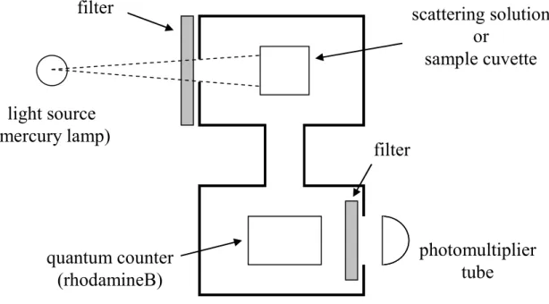
A schematic diagram of the apparatus used by Weber and Teale is shown in Figure I-4. Instead of the solid scatterer (MgO) used in the Vavilov method, Weber and Teale used solution scatterer (e.g. glycogen, colloidal silica). According to the Weber and Teale method, the Φf is given by Eq I-20

            + +       = Φ → → 2 s 2 e s e e s 0 0 f 3 3 ) ( ) ( 0 0 0 0 n n p p K K dA dE dA dS A A λ λ λ λ (I-20)

where e and s denote the sample emission and scattered light, respectively. The first term in Eq 20 is a direct measure of the intensity of the sample relative to the scattering solution. The second term corrects for the wavelength sensitivity of the detector. When a quantum counter is used, Ks/Ke can be assumed to be unity. The third term corrects for

anisotropy. The values pe and ps are the polarization degrees of scattered light and

emitted light, respectively. The last term corrects for refractive index differences between the sample and the standard solution. This method has the advantage that errors resulting from self-absorption and quenching of fluorescence can be eliminated by extrapolating measurements to zero concentration [7].

photomultiplier

tube

scattering solution

or

sample cuvette

quantum counter

(rhodamineB)

light source

(mercury lamp)

filter

filter

Figure I-4 Schematic diagram of an apparatus used in

the Weber and Teale method

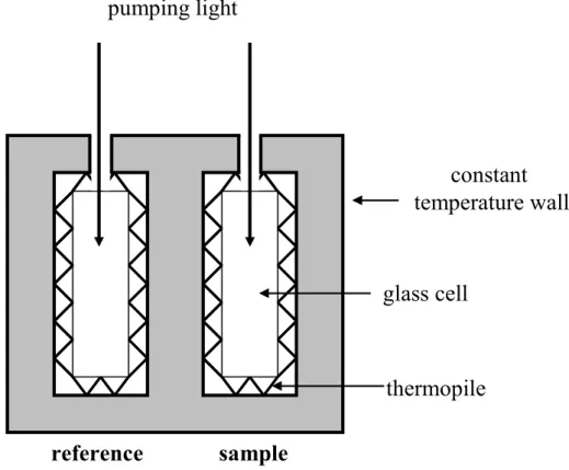
I-2-3 Calorimetric method

The calorimetric method determines the luminescence quantum yield of compounds by measuring heat energy released by nonradiative transitions against absorbed energy. The light energy absorbed by a sample solution may reappear in three forms: luminescence, chemical energy, and heat. In the absence of photochemical reactions, the yield of the luminescence is determined by obtaining the yield of heat. When a beam of light with energy E0 incidents upon a fluorescent sample, the sum of the transmitted

energy Et, the fluorescence energy Ef, and the heat energy Eh is equal to E0.

h f t

0 E E E

E = + + (I-21)

If Φh is the heat energy yield, then

t 0 h h E E E − = Φ (I-22)

The fluorescence quantum yield becomes

(

_h

)

f a f = 1−Φ Φ ν ν (I-23)

where

ν

a and

ν

f are the average energy of absorption and fluorescence, respectively.

compared with that of the reference solution. Since the reference solution has heat energy yield of unity, the ratio of the temperature rises gives the nonradiative yield which is the complement of the fluorescence energy yield. The calorimetric method is able to eliminate corrections for (1) anisotropic emission, (2) refraction of emitted light, (3) detection geometry and (4) detector response as a function of wavelength.

Figure I-5

Schematic diagram of an apparatus used in

the calorimetric method

thermopile

glass cell

constant

temperature wall

sample

reference

pumping light

I-3 Relative method

As described in I-2-1 and I-2-2, the absolute method requires various complex corrections to obtain Φf. Hence in most laboratories the quantum yield has been

measured by using the relative method in which the quantum yield is obtained by comparing the luminescence intensity of sample solution with that of standard solution. For dense sample solutions, the quantum yield is obtained by adopting the Vavilov configuration (the optically dense method). Using Eq I-16 the luminescence quantum yield (Φf) of sample solution is derived as

                  Φ = Φ ₂ r 2 f r f f r r f n n D D K K (I-24)

where Φr is the luminescence quantum yield of standard solutions. When a quantum

counter is used, Kr/Kf in Eq I-24 can be assumed to be unity, and Eq I-24then simplifies

to             Φ = Φ ₂ r 2 f r f r f n n D D (I-25)

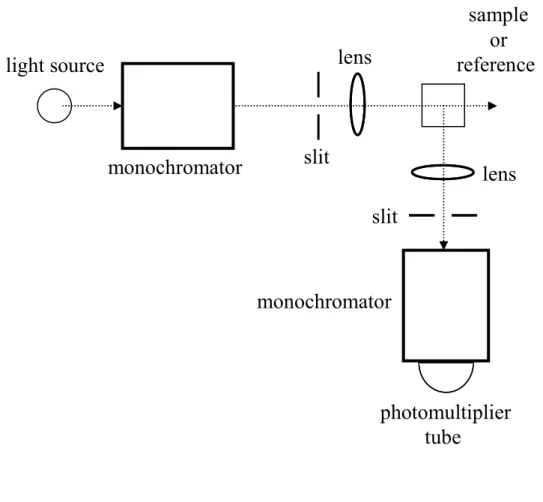
The luminescence quantum yield of dilute solution is obtained by using the spectrofluorometer as shown in Figure I-6 (the optically dilute method). In the optically dilute method, the luminescence quantum yield is given by Eq I-26

                  Φ = Φ ₂ r 2 f f r r f r f n n A A F F (I-26)

where f and r stand for the sample and standard reference, respectively, F is the integrated luminescence intensity, A is the absorbance of the solution. Usually sample solutions with sufficiently low concentrations (A < 0.1) are used in the optically dilute method. In order to obtain the accurate quantum yield, corrections for the refractive index is required. In the quantum yield measurements of the sample molecules in 77K rigid solution, it is necessary to take into account the additional corrections for optical anisotropy.

light source

Figure I-6 Schematic diagram of a spectrofluorometer

used in the relative method

photomultiplier

tube

monochromator

monochromator

_lens

lens

slit

slit

sample

or

reference

I-4 The purpose of this study

891011121314151617Recently, integrating sphere instruments [8-18] have received considerable attention

as they provide a simple and accurate means for determining the absolute luminescence quantum yield. By using an integrating sphere, much of the optical anisotropy is eliminated by multiple reflections on the inner surface of the integrating sphere. In the present thesis, a new apparatus to determine the absolute luminescence quantum yield of organic and inorganic molecules in solution at room-temperature and also in rigid solution at 77 K is developed by using an integrating sphere. Using this integrating sphere instrument, the absolute quantum yields of fluorescence standard solutions are reevaluated, and the fluorescence and phosphorescence quantum yields of 1-halogenated naphthalenes and 4-halobenzophenones in 77 K rigid solutions are measured to determine the rate constants for the spin-forbidden radiative and nonradiative transitions.

References

1 B. Valuer, Molecular Fluorescence Wiley-VCH: Weinheim, 2002.

2 J. R. Lakowicz, Principles of Fluorescence Spectroscopy, Springer, New York, ed. 3. 2006.

3 J. N. Demas, G. A. Crosby, J. Phys. Chem. 1971, 75, 991. 4 D. F. Eaton, Pure Appl. Chem. 1988, 60, 1107.

5 S. I. Vavilov, Z. Phys. 1924, 22, 266.

6 W. H. Melhuish, New Zealand J. Sci. Tech. 1955, 37, 142.

7 J. Adams, J. G. Highfield, G. F. Kirkbright, Anal. Chem. 1977, 49, 1850. 8 L. S. Rohwer, F.E. Martin, J. Lumin, 2005, 115, 77.

9 W. R. Ware, B. A. Baldwin, J. Chem. Phys. 1965, 43, 1194. 10 W. R. Ware, W. Rothman, Chem. Phys. Lett. 1976, 39, 449.

11 N. C. Greenham, I. D. W. Samuel, G. R. Hayes, R. T. Phillips, Y. A. R. R. Kessener, S. C. Moratti, A. B. Holmes, R. H. Friend, Chem. Phys. Lett. 1995, 241, 89.

12 J. C. de Mello, H. F. Wittmann, R. H. Friend, Adv. Mater. 1997, 9, 230.

13 H. Mattoussi, H. Murata, C. D. Merritt, Y. Iizumi, J. Kido, Z. H. Kafafi, J. Appl.

Phys. 1999, 86, 2642.

14 P. Mei, M. Murgia, C. Taliani, E. Lunedei, M. Muccini, J. Appl. Phys. 2000, 88, 5158.

15 L. F. V. Ferreira, T. J. F. Branco, A. M. B. Do Rego, ChemPhysChem, 2004, 5, 1848. 16 Y. Kawamura, H. Sasabe, C. Adachi, Jpn. J. Appl. Phys. 2004, 43, 7729.

17 L. Porrès, A. Holland, L. -O. Pålsson, A. P. Monkman, C. Kemp, A. Beeby, J. Lumin. 2006, 16, 267.

Chapter II

II-1 Absolute measurements of luminescence quantum yields using an integrating sphere

The fluorescence (Φf) and phosphorescence (Φp) quantum yields of solution samples

at room temperature were measured with an absolute photoluminescence quantum yield measurement system (Hamamatsu, C9920-02), which is shown schematically in Figure II-1. This system consists of a Xe arc lamp, a monochromator, an integrating sphere, a multichannel detector, and a personal computer. A 10 mm path length quartz cuvette for solution samples is set in the integrating sphere. A monochromatic light source was used as the excitation light source, which mounted a xenon lamp with the lamp rating of 150 W and an output stability of 1.0% (peak to peak). The excitation light was introduced into the integrating sphere by an optical fiber. The integrating sphere had an inner diameter of about 84 mm and contained a baffle between the sample and detection exit positions to prevent direct detection of the excitation light and/or emission from the sample. Spectralon (Labsphere) was mounted on the internal surface of the integrating sphere as a high reflectance material (99% reflectance for wavelengths from 350 nm to 1650 nm and over 96% reflectance for wavelengths from 250 nm to 350 nm).

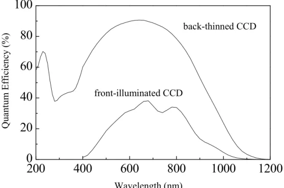
A photonic multichannel analyzer PMA-12 (Hamamatsu, C10027-01) was used as the multichannel detector. It employed a BT-CCD with 1024 × 122 pixels and a pixel size of 24 µm × 24 µm providing a wide spectrum range from 200 nm to 950 nm. Figure II-2 schematically shows the principle of a Czerny-Turner polychromator: the dispersion of the incident light by a grating and the detection of the dispersed light by a BT-CCD detector in PMA-12. The integrating sphere and the PMA-12 are connected by an optical fiber in which 15 core fibers are bundled. Figure II-3 illustrates the spectral response (without window) of front-illuminated CCD and BT-CCD. By using a BT-CCD, the sensitivity of the detector for fluorescence detection was vastly superior to

that of an optical detection system using a conventional CCD (i.e., a front-illuminated CCD), especially at short wavelengths.

The sensitivity of this system was fully calibrated for the spectral region 250−950 nm using deuterium and halogen standard light sources. These standard light sources were calibrated in accordance with measurement standards traceable to primary standards (national standards) located at the National Metrology Institute of Japan. The primary measurement standards are based onthe physical units of measurement according to the International System of Units (SI). The transfer accuracy in the sensitivity calibration was between ±2.4 and ±4.9%, depending on the wavelength.

The fluorescence quantum yield Φf is given by

( )

( )

[

]

( )

( )

[

]

∫

∫

− − = = Φ

λ

λ

λ

λ

λ

λ

λ

λ

d I I hc d I I hc sample ex reference ex reference em sample em PN(Abs) PN(Em) f (II-1)

where PN(Abs) is the number of photons absorbed by a sample and PN(Em) is the number of photons emitted from a sample,

λ

is the wavelength, h is Planck’s constant, c is the velocity of light, I_exsampleand I_exreference are the integrated intensities of the excitation light with and without a sample respectively, I_emsample and I_emreference are the photoluminescence intensities with and without a sample, respectively.

MC

PC

Xe

Lamp

Polychromator

BT-CCD

BF

OF

Integrating Sphere

SC

B

Figure II-1 Schematic diagram of an integrating sphere instrument

for measuring absolute luminescence quantum yields.

MC : monochromator, OF: optical fiber, BF : bundle

fiber, SC: sample cell, B: buffle, BT-CCD:

back-thinned CCD, PC: personal computer

Figure II-2 Optical arrangement of Czerny-Turner

polychromator combined with a BT-CCD

detector

(

(

concave mirror

concave mirror grating

BT-CCD plane mirror shutter slit Integrating Sphere MC Xe Lamp

PMA-12

bundle fiber

200

400

600

800

1000

1200

0

20

40

60

80

100

Q u an tu m E ff ic ie n cy ( % ) Wavelength (nm) front-illuminated CCD back-thinned CCD

Figure II-3 Spectral response (without window) of front-illuminated CCD

Figure II-4 shows the excitation light profile and the fluorescence spectra obtained by setting quartz cells with and without a sample solution, when a 1 N H2SO4 solution of

quinine bisulfate (QBS) is set inside the integrating sphere. The irradiation of a quartz cell that does not contain the sample solution gives the excitation light spectrum with a peak wavelength at 350 nm, and the excitation of the sample solution exhibits the fluorescence spectrum of QBS in the wavelength range 380 nm to 650 nm, which is accompanied by a reduction in the excitation light intensity. The spectra in Fig. II-4 are fully corrected for the spectral sensitivity of the instrument. The number of photons absorbed by QBS is proportional to the difference of the integrated excitation light profiles, while the number of photons emitted from QBS is proportional to the area under its fluorescence spectrum. Thus, according to Eq II-1, the fluorescence quantum yield can be calculated by taking the ratio of the difference of the integrated excitation light profiles to the integrated fluorescence spectrum.

II-2 Absorption and emission spectra

Absorption and emission spectra were measured with a UV/vis spectrophotometer (JASCO, Ubest-50) and a spectrofluorometer (Hitachi, F-4010), respectively. Rhodamine 6G/ethylene glycol solution was used for spectrum correction of the spectrofluorometer.

II-3 Fluorescence lifetime

Fluorescence decay times were determined with a time-correlated single-photon counting (SPC) fluorometer using a nanosecond flashlamp excitation source. For

QBS 400 450 500 550 600

300

400

500

600

700

800

Wavelength (nm) In te n si ty (a rb . u n it ) Reference QBS nm

Figure II-4

Excitation light profiles and fluorescence spectrum

obtained by 350 nm excitation of reference (solvent)

and quinine bisulfate (QBS) in 1N H

₂

SO

₄

. The inset

diagram of the system is shown in Figure II-5. A pulsed discharge lamp (pulse width ~1ns, repetition rate 40 kHz) filled with hydrogen gas was used as excitation light source. The emission light was detected by a photomultiplier tube (Hamamatsu, R955). The measured decay curves were analyzed on the basis of the deconvolution method. The instrumental pulse width of the apparatus was ~1 ns.

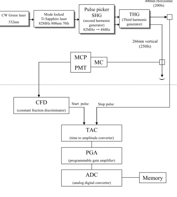
For picosecond lifetime measurements, the fluorescence decay curve was obtained by using the SPC system shown in Figure II-6. The picosecond lifetime measurements were carried out by using a self-mode-locked Ti:sapphire laser (Spectra-Physics, Tsunami; center wavelength 800 nm; pulse width ca. 70 fs; repetition rate 82MHz) pumped by a CW laser (Spectra-Physics, Millennia V; 532 nm; 4.5W). The second harmonic (400 nm, pulse width ca.200 fs) was generated by a sum frequency mixing of the fundamental and the second harmonic of the Tsunami laser system. The repetition frequency of the excitation pulse was reduced to 4MHz by using a pulse picker (Spectra-Physics Model 3980). The second harmonic (400 nm) in the output beam was used as trigger pulse. The emission light was detected by a microchannel plate photomultiplier (Hamamatsu, R3809U-51) after passing through a monochromator (Oriel, Model 77250). The instrumental response function had a half-width of 20-25 ps. The fluorescence time profiles were analyzed by iterative reconvolution with the response function.

The analysis of the fluorescence decay curve was carried out on the basis of the deconvolution method. Using the Instrumental response function I(t) and the fluorescence decay curve D(t) obtained by delta function excitation, the measured fluorescence decay curve F(t) is given by the following deconvolution integral:

t' ) t' ( ) t' t ( ) t ( t 0I D d F =

∫

− (II-2)

where I(t) was measured by using a scattering solution, and I(t) and F(t) were measured under the same experimental conditions. D(t) was used as a fitting function and assumed as the sum of exponential functions:

      − =

∑

i i i t exp ) t (

τ

B D (II-3)

where Bi and

τ

i are the preexponential factor and lifetime, respectively. Using Bi and

τ

i

as fitting parameters, the integral in Eq II-2 was calculated and least-square fitted to the observed fluorescence decay curve. Difference between the raw fluorescence data Y(t) and F(t) was evaluated by using the following equation:

2 2 min ) t ( ) t ( ) t (

∑

      − = t F Y σ χ (II-4)

Figure II-5

Schematic of time-correlated single photon counting

instrument used for fluorescence lifetime measurements

Start PMT Stop PMT Sample cell MC MC

p

p

nF900

decay Multiplexer Router CFD

(constant fraction discriminator)

TAC (time to amplitude converter)

MCA (multichannel analyzer)

CFD

(constant fraction discriminator)

p : polarizer MC : Monochromator

CFD

(constant fraction discriminator)

TAC

(time to amplitude converter)

CW Green laser 532nm CW Green laser 532nm Mode locked Ti:Sapphire laser 82MHz 800nm 70fs Mode locked Ti:Sapphire laser 82MHz 800nm 70fs Pulse picker SHG (second harmonic generator) 82MHz → 4MHz Pulse picker SHG (second harmonic generator) 82MHz → 4MHz THG (Third harmonic generator) THG (Third harmonic generator) 400nm Horizontal (200fs) 266nm vertical (250fs) MCP PMT MC Stop pulse Start pulse PGA

(programmable gain amplifier)

ADC (analog digital converter)

Memory

)

MCP-PMT : Microchannel PMT

Figure II-6 Schematic of picosecond time-resolved fluorometer based on

II-4 Transient absorption spectra

Transient absorption spectra were obtained by using a nanosecond laser flash photolysis system shown in Figure II-7. The third harmonic (355 nm, pulse width 4~6ns) or the fourth harmonic (266 nm, pulse width 3~5ns) of a Nd3+:YAG laser (Spectra-Physics, GCR－130) or XeCl excimer laser (Lambda Physik, LEXtra 50; 308 nm, pulse width ~17ns) was used as the excitation source. The monitoring light from a xenon lamp (Ushio, UXL-150D) was focused into a sample cuvette by two convex lenses. The transient signals were detected by a photomultiplier tube (PMT) after passing through a monochromator (MC), and recorded on a personal computer. In order to improve the signal to noise ratio (S/N) of the signal, the data averaging was carried out over 5 to 10 shots. The absorbance of each sample solution was adjusted to be ca. 0.7 at excitation wavelength. All sample solutions were degassed by the freeze-pump-thaw method.

The temperature control of the sample solution in the fluorescence lifetime measurements was made by using a cryostat (Oxford, DN1704) controlled with a temperature controller (Oxford, ITC503) or by using a constant temperature system (IWAKI, CTS-201).

II-5 Photoacoustic measurments

The experimental setup for time-resolved photoacoustic spectroscopy system is shown in Figure II-8. Photoacoustic (PA) measurements were made by using the third harmonic (355 nm) of a Nd3+:YAG laser as the excitation source. The sample solution was irradiated by the laser beam after passing through a slit (0.5 mm width). The

Figure II-7 Schematic of nanosecond laser photolysis system

Nd

3+

_{:YAG Laser}

Nd

3+

_{:YAG Laser}

Xe lamp

_MC

_PMT

PD

Personal

computer

Timing

Circuit

Sample

cell

MC : monochromator

PMT : photomultiplier tube

Digital Storage

Oscilloscope

Dichroic mirror Dichroic mirror

pyroelectiric energy meter (Laser Precision, Rjp-753 and Rj-7610). The PA signals detected by a piezoelectric detector (panametrics V103, 1MHz and panametrics M109, 5MHz) were amplified by using a wide-band high-input impedance amplifier (panametrics 5675, 50 kHz, 40 dB) and fed to a digitizing oscilloscope (Tektronix, TDS-540). The temperature of the sample solution was held to ± 0.02 K.

The intensity (H) of photoacoustic signal can be expressed as

(

)

L A _E

H =K

α

1−10− (II-5)

where K is a constant containing the thermoelastic properties of the solution and instrumental factors, EL is the laser pulse fluence, A is the absorbance of the sample

solution and

α

is the fraction of energy deposited in the medium as prompt heat within the time resolution of the experiment [1,2]. The theoretical background of photoacoustic spectroscopy is described in Appendix. Figure II-9a shows the photoacoustic signals taken for 2-hydroxybenzophenone (2HBP) in acetonitrile (CH3CN) at 293 K. As shown

in Figure II-9b signal amplitude plotted against the laser fluence gave a straight line. Since it is known that the α value for the reference compound (2HBP) can be assumed to be unity, one can determine the α value of the sample compound by calculating the ratio of the slopes of the straight lines.

Trigger Iris (1mm) ND filter Beam splitter Power probe Power meter Slit (0.5mm) Dichroic mirror Dichroic mirror Digitizing oscilloscope Preamplifier Computer Sample Cell Nd3+_{:YAG Laser} Piezoelectric detector (Panametrics V103)

Figure II-8 Schematic of time-resolved photoacoustic

spectroscopy (PAS) instrument

0 20 40 0 0.1 0.2 0 5 10 –0.02 0 0.02

Time (µs)

P

A

s

ig

n

al

(

ar

b

.

u

n

it

)

(a)

(b)

P

A

s

ig

n

al

a

m

p

li

tu

d

e

Laser fluence (µJ)

Figure II-9 (a) Laser fluence dependence of PA signals for 2HBP

in CH

₃

CN (b) PA signal amplitude as a function of

laser fluence for 2HBP in CH

₃

CN (E

_λ

= 355 nm)

Appendix Theory

Photoacoustic spectroscopy is based on the absorption of light, leading to the local warming of the absorbing volume element. The subsequent expansion of the volume element generates a pressure wave proportional to the absorbed energy, which can be detected by pressure detectors [1,2]. Rothberg and co-workers [3] initially modeled the photoacoustic experiment with a point source of heat given the analytical form (1/τ)exp(-t/τ), where τ is the lifetime of the transient and the preexponential term 1/τ is a normalization factor so that the total heat deposition of transient is independent of τ. The pressure transducer signal reflects the original heat deposition profile in space and time. Local thermal expansion initiates acoustic waves that obey the wave equation

( )

( )

h

( )

r t t t r P v t r P s , 4 , 1 , ₂ 2 ₌₋ ′ ∂ ′ ∂ − ′ ∇ π (II-6)

where h(r’,t) is heat source function, r’ and t refer to the spatial and temporal source coodinate, vS is the speed of sound in the medium and P(r’,t) is the wave amplitude at

the observer’s coordinate r’, t. when h(r’,t) is assumed to be an impulse source as the spread of the sound in spherical symmetry field, the wave amplitude P(r’,t) at the detector is given by

( )

( )τ τ π / / 0 0 0 0 1 4 , _e t r vs r h t r P = − − (II-7)

converts P(ro,t) to an electrical signal. The transducer such as PZT was defined to be

sensitive to longitudinal displacement waves and was modeled as an underdamped harmonic oscillator whose impulse response is.

( )

_{, sin}

(

(

)

)

τ0 t t e t t v A t t G ′ − − ′ − = ′ (II-8)

where G(t,t’) is Green’s function for the transducer, v is the characteristic oscillation frequency of the transducer. The detector response V(t) for an arbitrary forcing function

P(r0,t) is given by convolving the impulse response with the forcing function:

( )

t G

( ) (

t t P r t

)

dt V =

∫

t ′ ′ ′

∞

− , 0, (II-9)

Thus, the photoacoustic waveforms (time domain convolution of the heat source and detector) can be modeled according to the following equation

( )

(

′

)

− 

( )

− ′

( )

 + = − − vt v vt e e v v r A h t V t t sin 1 cos / 1 / 4 0 2 2 0 0

τ

τ

τ

π

τ τ _(II-10)

where V(t) is the detector response, h0A/πr0 is constant, v is the characteristic oscillation

frequency of the transducer,

τ

0 is the relaxation time of the transducer,

τ

is the transient,

( )

(

)

( )

( )

_            ′ − − ′ + ′ = − − =

∑

vt v vt e e v v K t V k t t k k n k k k _cos 1 _sin / 1 / ₀ 2 2 1

τ

τ

τ

φ

τ τ (II-11)

where K' is constant,

φ

k is amplitude factor for transient k,

φ

k is lifetime of transient k,

and 1/

τ

’ = 1/

τ

– 1/

τ

0. Eq II-11 means that the observed acoustic wave resulting from

the heat depositions of several simultaneous decays is the sum of the waveforms which would be observed from each of the decays individually.

Photoacoustic signal measurement

For photochemically simple systems with known quantum yield and kinetics, the amplitude of photoacoustic signal is related to the energy of the incident laser pulse by [5]

(

)

L A

E

H =K

α

1−10− (II-12)

where H is the experimentally obtained amplitude of the acoustic signal, K is instrumental constant which depends on the geometry of the experimental set-up and the thermoelastic quantities of the medium, EL is the incident laser pulse energy, A is the

optical density of the solution, and

α

is the fraction of the absorbed laser energy (Eabs)

released as thermal energy (Eth) with the response time of the detector (prompt heat),

and given by abs th E E = α (II-13)

where 0 ≤

α

≤ 1. The application of Eq II-12 supposes a cylindrical acoustic wave. H is used to determine the fraction of the heat stored by species with

τ

nr longer than the

experimental time resolution of the instrument. In order to eliminate K, a calorimetric reference with

α

= 1 is needed. Using a calorimetric reference with

α

=1, the value of

α

for the sample is given by the ratio H/EL for sample and reference.

Heat integration time

The probable origin for the lower limit is that the measurements are ultimately limited by the acoustic transit time (

τ

a) of the PAS apparatus. This parameter is defined

as a a V R =

τ

(II-14)

where

τ

a is the time required by the acoustic wave to travel across the laser beam radius,

R is the radius of the excitation beam and Va is the velocity of sound in the sample

medium . Assuming that the beam radius is 0.5 mm and a velocity of sound in water is 1470 ms-1 at 293K, the acoustic transit time becomes 340ns.

References

[1] Braslavsky, S. E.; Heibel, G. E. Chem. Rev. 1992, 92, 1381.

[2] Braslavsky, S. E.; Heihoff, K. In Handbook of Organic Photochemistry, Scaiano, J. C., Ed., CRC Press: Boca Raton, FL1989; Vol. 1, p327.

[3] Rothberg, L. J.; Simon, J. D.; Bernstein, M.; Peters, K. S.; J. Am. Chem. Soc. 1983, 105, 3464.

[4] Rudzki, J. E.; Goodman, J. L.; Peters, K. S. J. Am Chem. Soc.1985, 107, 7849 [5] (a) Braslavsky, S. E.; Heibel, G. E. Chem. Rev. 1992, 92, 1381. (b) Churio, M. S.;

Angermund, K. P.; Braslabsky, S. E. J. Phys. Chem. 1994, 98, 1776. (c) Gensch, T.; Braslabsky, S. E. J. phys. Chem. B 1997, 101, 101. (d) Small J. R. Libertini, L. J.; Small, E. W. Biophys. Chem. 1992, 42, 29. (e) Borsarelli, C. D.; Bertolotti, S. G.; Previtali, C. M. Photochem. Photobiol. Sci, 2003, 2, 791.

Chapter III

Absolute Measurements of Luminescence

Quantum Yield of solutions at Room

III-1 Introduction

As described in Chapter I the absolute methods require performing various complex corrections to obtain accurate quantum yields. Therefore, in most laboratories relative (secondary) methods are used to determine quantum yields. In the relative methods, the quantum yield of a sample solution is determined by comparing the integrated fluorescence intensity with that of a standard solution under identical conditions of incident irradiance. Thus, it is critical to correct for the spectral sensitivity of the instrument, and the measured quantum yield is only as accurate as the certainty of the quantum yield of the fluorescence standard. One of the most widely used secondary standards is quinine bisulfate (QBS) in 1 N H2SO4 at 298 K (Φf = 0.546 for infinite

dilution) reported by Melhuish [1,2]. This value was estimated by extrapolating the Φf

value (0.508) of 5.0 × 10-3 M QBS solution, which was determined by absolute measurements based on the modified Vavilov method, to infinite dilution using the self-quenching constant [1]. There is a limited amount of data available for such a widely used reference [3-8]. 9,10-Diphenylanthracene (DPA) has also been employed as a popular fluorescence standard because of its high quantum yield. However, the published quantum yields of DPA vary widely from 0.86 to 1.06 [9-13].4567891011121314151617181920212223

As described in Chapter II, integrating sphere instruments [8, 14-23] provide a simple and accurate means for determining the absolute luminescence quantum yield. By using an integrating sphere, much of the optical anisotropy is eliminated by multiple reflections on the inner surface of the integrating sphere. A new instrument for determining the absolute luminescence quantum yield of solutions, solids [24], and thin films [24] has been developed by utilizing an integrating sphere for a sample chamber to eliminate the effects of polarization and refractive index from measurements. In Chapter III, The absolute quantum yields of representative fluorescent standard solutions are

reevaluated by using the integrating sphere instrument.

III-2 Materials

Figures III-1 and III-2 show the sample molecules used in this chapter. 2-Aminopyridine (2-APY; Tokyo Kasei) was purified by recrystallization from cyclohexane. Quinine bisulfate (QBS; Wako) was purified by recrystallization three

times from water. 3-Aminophthalimide (3-API; Kodak) and

N,N-dimethylamino-m-nitrobenzene (N,N-DMANB; Tokyo Kasei) were purified by recrystallization from ethanol. 4-Dimethylamino-4’-nitrostilbene (4,4’-DMANS; Tokyo Kasei) was purified by recrystallization from chloroform. Naphthalene (Kanto) and 1-aminonaphthlene (Tokyo Kasei) were purified by vacuum sublimation. Anthracene (Tokyo Kasei) was purified by recrystallization from ethanol. 9,10-Diphenylanthracene (DPA; Lancaster) was purified by high-performance liquid chromatography.

N,N-Dimethyl-1-aminonaphthalene (Kanto) was purified by distillation under reduced pressure. Fluorescein (Wako) was purified by column chromatography on a silica-gel column using ethyl acetate as the eluent. Tryptophan (Kanto) was used as received. Cyclohexane (Aldrich, spectrophotometric grade), ethanol (Tokyo Kasei, spectrophotometric grade), sulfuric acid (Wako, analytical grade), benzene (Kishida, spectrophotometric grade) and o-dichlorobenzne (Kishida) were used without further purification.

N NH2 O O NH NH2 NO2 N O2N N N O HO N OH S O O OH

2-Aminopyridine

(2-APY)

Quinine bisulfate

(QBS)

3-Aminophthalimide

(3-API)

N,N-dimethylamino-m-nitrobenzene

(N,N-DMANB)

4-Dimethylamino-4’-nitrostilbene

(4,4’-DMANS)

NH2 N HO O O COOH NH2 N H O OH

Figure III-2 Structures of compounds used in chapter III

Naphthalene

Anthracene

N,N-Dimethyl-1-aminonaphthalene

1-Aminonaphthlene

9,10-Diphenylanthracene

(DPA)

Fluorescein

Tryptophan

III-3 Results and Discussion

III-3-1 Spectral sensitivity of instrument

In the absolute fluorescence quantum yield measurements using an integrating sphere, the obtained absorption and fluorescence spectra of the sample solutions need to be corrected for the spectral sensitivity of the entire system, including the integrating sphere, the grating monochromator, and the photon detector. Thus, the spectral sensitivity of our instrument was calibrated both for an integrating sphere and a multichannel spectrometer by using deuterium and halogen standard light sources. Using the calibrated multichannel spectrometer (without the integrating sphere), we first remeasured the absolute fluorescence spectra of some standard solutions: 2-APY (10-5 M in 0.1 N H2SO4), QBS (10-5 M in 0.1 N H2SO4), 3-API (5 × 10-4 M in 0.1 N H2SO4), N,N-DMANB (10-4M in benzene:hexane (3:7, v/v)), and 4,4’-DMANS (10-3 M in

o-dichlorobenzene) [ 25 ]. The normalized fluorescence spectra of these standard solutions are displayed in Figure III-3 together with the data from the literature. [24,26] Good agreement was obtained for 2-APY, QBS, and 3-API, while a significant difference is found for the long wavelength region, i.e., the near-infrared region of

N,N-DMANB and 4,4’-DMANS. Because our instrument uses a BT-CCD as the photon detector, its sensitivity in the near-infrared region is significantly better than that of a conventional photomultiplier tube. A complete set of corrected spectra (in relative quanta per wavelength) is summarized in Table III-1.

Then the fluorescence spectra of these standard solutions were measured by using the entire system (including the integrating sphere). The corrected spectra agreed very closely with those obtained by the multichannel spectrometer, indicating that the spectral sensitivity of the whole system including the reflectivity of the integrating sphere is properly corrected in the spectral region 250-950 nm.

Wavelength (nm)

In

te

n

si

ty

(a

rb

.

u

n

it

)

2-APY QBS 3-API N,N-DMANB 4,4’-DMANS

300

0

400

500

600

700

800

900

50

100

Figure III-3 Corrected fluorescence spectra for 2-APY (10

–5

_{M in 0.1 N}

H

₂

SO

₄

), QBS (10

–5

_{M in 0.1 N H}

2

SO

4

), 3-API (5×10

–4

M in

0.1 N H

₂

SO

₄

),N,N’-DMANB (10

–4

_{M in benzene-hexane (3:7,}

v/v)), and 4,4’-DMANS (10

–3

_{M in o-dichlorobenzene）.}

λ (nm) λ (nm) λ (nm) λ (nm) I (λ) λ (nm) 300 1.2 322.6 4.9 380 0.8 635 1.8 384.6 1.4 305 1.0 331.7 14.9 385 1.6 640 1.7 388.3 3.5 310 2.0 346.0 66.3 390 3.0 645 1.5 392.2 5.5 315 2.2 359.7 98.1 395 6.0 650 1.3 396.0 8.7 320 4.4 367.7 100 400 11.6 655 1.0 400.0 13.8 325 10.5 375.9 91.8 405 21.4 660 1.2 404.0 19.4 330 23.9 390.6 66.0 410 33.0 665 0.8 408.2 26.6 335 41.2 404.9 37.1 415 46.2 670 0.8 412.4 36.6 340 56.5 420.2 20.2 420 59.3 675 0.7 416.7 45.5 345 73.2 434.8 9.5 425 71.2 680 0.8 421.1 54.7 350 85.9 450.5 4.9 430 80.7 685 0.5 425.5 64.6 355 95.3 465.1 2.4 435 88.9 690 0.7 430.1 74.6 360 98.9 480.8 0.6 440 93.2 695 0.4 434.8 82.5 365 98.9 445 97.7 700 0.6 439.6 90.0 370 96.3 450 99.4 444.4 95.0 375 91.1 455 99.9 449.4 98.6 380 83.4 460 98.6 454.5 100 385 73.6 465 95.5 459.8 99.2 390 65.7 470 90.9 465.1 97.5 395 56.9 475 86.8 470.6 93.8 400 48.5 480 81.9 476.2 88.3 405 41.9 485 76.1 481.9 81.7 410 35.2 490 70.0 487.8 74.9 415 29.8 495 63.8 493.8 67.9 420 24.9 500 58.1 500.0 60.3 425 20.4 505 52.4 506.3 53.4 430 16.8 510 47.1 512.8 46.9 435 13.7 515 42.1 519.5 41.0 440 10.8 520 37.4 526.3 35.0 445 9.3 525 33.3 533.3 30.0 450 7.4 530 29.5 540.5 24.9 455 6.1 535 26.0 547.9 20.0 460 5.2 540 22.8 555.6 16.4 465 4.3 545 20.2 563.4 13.6 470 3.4 550 17.5 571.4 11.6 475 2.8 555 15.3 579.7 10.0 480 2.4 560 13.5 588.2 8.5 485 1.8 565 12.0 597.0 6.8 490 1.8 570 10.3 606.1 5.5 495 1.2 575 9.0 615.4 4.2 500 1.1 580 7.9 625.0 3.2 505 1.0 585 6.9 634.9 2.4 510 0.8 590 5.9 645.2 1.5 515 0.5 595 5.4 655.7 0.7 520 0.3 600 4.6 666.7 0 525 0.6 605 3.9 530 0.2 610 3.6 535 0.1 615 3.2 540 0.1 620 2.7 545 0.4 625 2.4 550 0.1 630 2.3 I (λ) I (λ) I (λ) I (λ) 2-APY QBS

this work literature this work literature

λ (nm) λ (nm) I (λ) λ (nm) λ (nm) λ (nm) 420 0.4 675 3.3 434.8 1.4 425 0.3 680 16.7 444.4 2.2 425 0.5 680 3.0 439.6 2.0 430 0.8 685 15.6 449.4 2.9 430 0.8 685 2.7 444.4 4.0 435 1.3 690 14.2 454.5 4.2 435 1.5 690 2.3 449.4 7.7 440 1.5 695 12.4 459.8 8.3 440 2.6 695 2.1 454.5 13.9 445 2.0 700 11.8 465.1 14.2 445 5.1 700 1.9 459.8 21.5 450 3.9 705 10.7 470.6 21.1 450 9.2 705 1.7 465.1 33.7 455 6.7 710 9.5 476.2 30.2 455 15.5 710 1.5 470.6 46.4 460 10.3 715 8.7 481.9 40.8 460 24.3 715 1.3 476.2 60.8 465 15.2 720 8.7 487.8 50.9 465 34.9 720 1.2 481.9 74.0 470 22.4 725 7.1 493.8 61.0 470 47.0 725 1.0 487.8 84.8 475 30.7 730 6.8 500.0 71.2 475 59.5 730 1.0 493.8 93.4 480 38.8 735 6.2 506.3 81.4 480 71.5 735 0.8 500.0 98.4 485 47.9 740 5.6 512.8 88.7 485 82.1 740 0.7 506.3 100 490 57.0 745 4.8 519.5 94.1 490 90.0 745 0.7 512.8 99.0 495 64.8 750 5.2 526.3 98.5 495 95.4 750 0.6 519.5 95.0 500 72.3 755 4.3 533.3 100.0 500 99.0 755 0.4 526.3 89.2 505 79.5 760 3.5 540.5 99.3 505 99.9 760 0.5 533.3 82.3 510 85.8 765 3.6 547.9 96.7 510 99.5 765 0.5 540.5 73.5 515 89.9 770 3.1 555.6 92.2 515 97.3 770 0.3 547.9 63.3 520 93.9 775 2.9 563.4 87.3 520 93.6 775 0.3 555.6 54.8 525 96.9 780 2.9 571.4 81.8 525 89.4 780 0.4 563.4 46.3 530 99.0 785 3.0 579.7 75.5 530 84.6 571.4 39.9 535 99.4 790 2.2 588.2 69.6 535 79.1 579.7 34.1 540 99.3 795 1.9 597.0 63.8 540 73.3 588.2 29.0 545 98.1 800 2.2 606.1 58.0 545 67.1 597.0 24.5 550 95.7 805 2.2 615.4 52.4 550 61.3 606.1 20.9 555 93.4 810 0.9 625.0 45.9 555 55.9 615.4 17.5 560 90.6 815 1.7 634.9 40.2 560 50.7 625.0 14.7 565 87.3 820 1.3 645.2 35.0 565 45.8 634.9 12.3 570 82.5 825 2.3 655.7 30.5 570 40.9 645.2 10.0 575 79.1 830 0.4 666.7 26.6 575 36.6 655.7 7.9 580 75.3 835 1.7 678.0 22.5 580 32.8 666.7 5.9 585 70.7 840 1.1 689.7 19.0 585 29.1 678.0 4.2 590 66.3 701.8 16.3 590 25.8 689.7 2.7 595 62.4 714.3 13.4 595 22.9 701.8 1.6 600 58.8 727.3 11.0 600 20.4 714.3 0.8 605 54.7 740.7 9.0 605 17.9 610 50.9 754.7 6.9 610 15.9 615 47.7 769.2 5.4 615 14.2 620 44.1 784.3 4.0 620 12.5 625 40.9 800.0 2.7 625 11.1 630 37.9 816.3 1.8 630 9.8 635 35.3 833.3 0.8 635 8.7 640 32.2 640 7.6 645 29.8 I (λ) λ (nm) I (λ) I (λ) I (λ) I (λ) 3-API N,N -DMANB

this work literature this work literature

λ (nm) λ (nm) 550 0.3 795 51.2 555.6 2.6 555 0.5 800 48.1 563.4 3.4 560 1.0 805 45.3 571.4 4.1 565 1.4 810 41.9 579.7 6.4 570 2.1 815 39.9 588.2 9.4 575 3.3 820 36.7 597.0 13.6 580 4.9 825 34.7 606.1 19.1 585 6.6 830 32.9 615.4 24.9 590 8.8 835 30.6 625.0 33.2 595 11.6 840 28.7 634.9 42.8 600 14.8 845 26.4 645.2 53.2 605 18.4 850 24.6 655.7 64.0 610 22.7 855 23.1 666.7 74.7 615 27.0 860 20.8 678.0 84.5 620 32.0 865 18.8 689.7 91.9 625 37.6 870 17.9 701.8 96.4 630 43.2 875 16.8 714.3 99.4 635 49.0 880 15.9 727.3 100.0 640 55.2 885 14.8 740.7 98.4 645 60.8 890 13.4 754.7 93.3 650 66.6 895 12.8 769.2 86.7 655 72.1 900 11.9 784.3 78.1 660 77.1 905 10.8 800.0 67.9 665 82.1 910 10.2 816.3 57.1 670 86.4 915 9.5 833.3 46.6 675 90.3 920 8.5 851.1 37.6 680 93.6 925 8.3 869.6 29.6 685 96.1 930 7.5 888.9 22.2 690 98.8 935 6.9 909.1 16.0 695 99.4 940 6.9 930.2 11.5 700 100 945 6.2 952.4 7.4 705 99.6 950 5.7 710 99.1 715 98.2 720 96.9 725 95.0 730 91.8 735 89.8 740 87.8 745 84.9 750 81.2 755 78.5 760 74.7 765 71.2 770 67.7 775 64.6 780 60.7 785 57.9 790 54.4 I (λ ) λ (nm) I (λ ) I (λ )

this work literature

4,4'-DMANS

III-3-2 Effects of reabsorption and reemition

The fluorescence spectrophotometer equipped with an integrating sphere is useful for compensating the effects of polarization and refractive index in the quantum yield measurements. However, random and multiple scattering of excitation light on the inner wall of the integrating sphere increases the effective optical path length. This increases the effect of reabsorption and reemission on quantum yield measurements, especially in compounds whose absorption and fluorescence bands substantially overlap.

In order to clarify the effects of reabsorption and reemission on the quantum yield obtained using our integrating sphere instrument, the influence of the concentration of anthracene in ethanol on the fluorescence spectrum and quantum yield was examined. The anthracene concentration was varied between 1.0 × 10-6 M and 1.0 × 10-3 M at room temperature. The absorption and fluorescence spectra of anthracene overlap significantly with each other in the 0-0 band region.

As shown in Figure III-4, the 0-0 vibrational band around 375 nm is almost absent in the fluorescence spectrum of 1.0 × 10-3 M solution when the integrating sphere is used. When the concentration is reduced, the intensity of the 0-0 band increases remarkably and reaches a maximum at a concentration of 1.0 × 10-6 M. The fluorescence spectrum of the 1.0 × 10-6 M solution obtained using the integrating sphere instrument was in almost consistent with that obtained using a conventional fluorescence spectrophotometer. The observed Φf values (Φ ) varied from 0.278 for a 1.0 × 10obsf

-5

M solution to 0.220 for a 1.0 × 10-3 M solution (see Table III-2).

300

400

500

Wavelength (nm)

1.0×10-6_M 1.0×10-5 5.0×10-5 1.0×10-4 5.0×10-4 1.0×10-3

Abs.

Fluo.

A

b

so

rb

an

ce

(a

rb

.

u

n

it

)

In

te

n

si

ty

(a

rb

.

u

n

it

)

In

te

n

si

ty

(a

rb

.

u

n

it

)

Wavelength (nm)

(a)

(b)

400

500

Figure III-4 (a) Absorption and fluorescence spectra of 1.0×10

–6

_M

anthracene in ethanol, and (b) concentration dependence

of the fluorescence spectra of anthracene in ethanol

a

a

a

a

1.0 × 10

-5

0.278

0.066

0.290

0.972

0.099

0.975

5.0 × 10

-5

0.262

0.142

0.294

0.966

0.173

0.971

1.0 × 10

-4

0.252

0.179

0.291

0.963

0.215

0.971

5.0 × 10

-4

0.235

0.251

0.289

0.963

0.299

0.973

1.0 × 10

-3

0.220

0.271

0.280

0.962

0.327

0.974

concentration

(M)

anthracene

DPA

obs f

Φ

Φ

_f obs f

Φ

Φ

f

Table III-2 Observed and Corrected Fluorescence Quantum Yields

of Anthracene in Ethanol and DPA in Cyclohexane

To correct the effect of reabsorption and reemission, the method recently reported by Ahn et al. [27] was used. They considered a fluorescent system with a quantum yield of Φf. If the probability of an emitted photon being reabsorbed by sample molecules is expressed by a (see Figure III-5), the photon escape probability is given by 1-a. The observed fluorescence quantum yield Φ is then given by the geometric series obs_f

We used f f 2 f 2 f f obs f 1 ) 1 ( ) 1 )( 1 ( Φ − − Φ = ⋅ ⋅⋅ + Φ + Φ + − Φ = Φ a a a a a (III-1)

where the successive terms represent photon escape after successive absorption−reemission cycles. The self-absorption parameter a depends on the overlap between the absorption and fluorescence spectra, and can be estimated by comparing the observed fluorescence spectrum with that of a sufficiently diluted solution (the true fluorescence spectrum) using the following equation [27].

( )

( )

∫

∫

− = dλ λ I dλ λ I a obs 1 (III-2) where

∫

Iobs

( )

λdλ

f represents the area (integrated intensity) of the observed

fluorescence spectrum, and

∫

I_f

( )

λ dλ denotes the area of the true fluorescence spectrum without reabsorption (see Figure III-5). An equation for calculating the fluorescence quantum yield can be derived from Eq III-1 and is given by

Wavelength (nm)

400

500

400

500

Absence of fluorescence

by reabsorption

Figure III-5 Fluorescence spectra of 1.0×10

-3

_{M anthracene}

in ethanol used for the calculation of a

In

te

n

si

ty

(a

rb

.

u

n

it

)

obs f obs f f 1− + Φ Φ = Φ a a (III-3)

Table III-2 presents the fluorescence quantum yields of anthracene solutions corrected for reabsorption/reemission effects using Eq III-3 along with the values of the self-absorption parameter a and the uncorrected quantum yieldΦ . The corrected Φobs_f f gives almost constant values in the concentration range 1.0 × 10-5 M to 1.0 × 10-3 M. This correction method is thus useful for determining the Φf value of high-concentration sample solutions.

28

III-3-3 Fluorescence quantum yields of standard solutions

The quantum yields of representative fluorescence standard compounds dissolved in organic solvents or H2O obtained using our instruments are shown in Table III-3 along with accepted values from the literature. The compounds in Table III-3 are commonly used as fluorescence standards in quantum-yield measurements based on a relative (secondary) method with optically dilute or dense solutions [29,30]. Because the magnitude of the fluorescence quantum yield depends on the physical conditions, such as the solvent, the sample concentration, and the excitation wavelength, these parameters are also specified in Table III-3. Inspection of the Φf values in Table III-3 reveals that there is excellent agreement between our Φf values and the values given in the literature and that they lie within experimental errors, with the exception of DPA in cyclohexane and 1.0 × 10-5 M QBS in 1 N H2SO4 aqueous solution.

Table III-3 Comparison of Φ_fValues of Some Fluorescence Standard Solutions Obtained in This Study with Values from the Literature

compound solvent conc. (M) λexc (nm)

a _Φ f (literature) naphthalene cyclohexane 7.0 × 10-5 270 0.23 ± 0.01 0.23 ± 0.02 [30] anthracene ethanol 4.5 × 10-5 340 0.28 ± 0.02 0.27 ± 0.03 [30] DPA cyclohexane 2.4 × 10-5 355 0.97 ± 0.03 0.9 ± 0.02 [11] 1-aminonaphthalene cyclohexane 5.7 × 10-5 300 0.48 ± 0.02 0.465 [28] N,N -dimethyl-1- cyclohexane 1.0 × 10-4 300 0.011 ± 0.002 0.011 [28] aminonaphthalene quinine bisulfate 1N H2SO4 5.0 × 10-3 350 0.52 ± 0.02 0.508 [1] 1N H2SO4 1.0 × 10-5 350 0.60 ± 0.02 0.546 [1] fluorescein 0.1N NaOH 1.0 × 10-6 460 0.88 ± 0.03 0.87b [3] tryptophan H2O (pH 6.1) 1.0 × 10 -4 270 0.15 ± 0.01 0.14 ± 0.02 [29] Φf (this work) a