トップページ - 横浜国立大学学術情報リポジトリ

全文

(1)研究ノート. . A didactic note on the use of Benford’ s Law in public works auditing, with an application to the construction of the Brazilian“Amazon Arena” 2014 World Cup soccer stadium 1） Mauricio Soares Bugarin and Flavia Ceccato Rodrigues da Cunha. Abstract. Globalization requires developing countries’ governments to invest heavily in expensive large-scale infrastructure projects in order to keep on the map of an ever more competitive world. In a context of capital constraint, it is essential to keep public procurement works at their lowest possible cost while assuring a high quality output. This paper introduces Benford’ s Law as a tool to detect overpricing in worksheets of public works. That law suggests that the frequency of the first digit in a multitude of non-manipulated numerical databases decreases successively from digit 1 (about 30%) to digit 9 (less than 5%). The paper describes a few relevant statistical tests of Benford’ s Law and applies them to the construction work of Brazil’ s Amazon Arena 2014 World Cup soccer stadium. Then, it compares Benford’ s Law results with those obtained from the analysis of prices conducted by the Brazilian Court of Accounts (TCU). The tests identified items in the worksheet that did not comply with the Law and corresponded to over 80% of the total overprice uncovered by TCU. That identification required auditing only 65% of total procurement costs, whereas the methodology used by TCU audited about 80% of total costs. Finally, we propose an alternative algorithm for selecting the sample to be audited while still auditing the conventional 80% of total costs. Keywords: Audit. Public works. Benford’ s Law. Overpricing. Public expenditure. 1. Introduction. This paper is concerned with the challenge of controlling public expenditure in modern economies. More specifically, it focuses on the auditing process of large government procurements and presents a novel methodology to guide the selection of items to be audited for possible prices set above competitive benchmarks. The methodology is based on a statistic regularity called“Benford’ s Law", which states that in large natural, no-manipulated numerical databases the occurrence of the first digit of the numbers are decreasing from 1 to 9, in such a way that 1 appears as the leading digit of about 1）The authors are grateful to Brian Gaines for introducing Benford’ s Law, to Adriana Portugal and, most especially, to Keiichi Yamazaki for discussions, comments and encouragements. The authors. remain sole responsible for opinions expressed, remaining errors or omissions. Mauricio Bugarin gratefully acknowledges the Brazilian National Research Council, CNPq, research grant.. 『エコノミア』第 66 巻第 1 号（2015 年 5 月），23-55 頁［Economia Vol. 66 No.1（May 2015），pp. 23-55］.

(2) . 30% of all numbers, 2 appears as the leading digit of about 15% of all numbers, and so on until 9, which appears as the first digit of less than 5% of all numbers. The main idea behind the use of that statistical law is that if a database is manipulated by human intervention, then it is less likely that it will follow Benford’ s Law. This paper applies the methodology based on Benford’ s Law to highlight which item categories should be audited. Then it compares these suggestions with the auditing of the“Amazon Arena” Soccer Stadium performed by the Brazilian Federal Court of Accounts, the TCU, based on that institution’ s own methodology. The comparison shows that the methodology based on Benford’ s Law was able to uncover 80% of the total overpricing found by the TCU, while suggesting the auditing of only 65% of the total budget. The article is organized as follows. First, section 2 discusses Benford’ s Law in more detail. Then, section 3 briefly introduces the“Amazon Arena”soccer stadium that was built as a government procurement project for the 2014 FIFA World Soccer Cup competition. Section 4 describes the tests inspired on Benford’ s Law that we will use in order to determine evidence of overpricing in the winning bid for the construction of the stadium. Section 5 applies these tests to the original winning worksheet of the Amazon Arena. Section 6 compares the evidence suggested by our tests with the Brazilian Federal Court of Accounts, the TCU’ s audit and section 7 suggests a new algorithm for selecting the auditing sample of a large procurement worksheet. Finally, section 8 presents our conclusions.. 2. Benford’s Law. According to Japan Statistics Bureau, in 2010 the country had 1751 municipalities where lived a 2）. total population of 128,057,352 people . Consider a database composed of each one of the cities’ 3）. populations; then calculate the number of cities whose population count’ s first digit is 1, such as the city of Kyoto, 1,474,015 inhabitants or Tarumisu, in Kagoshima, with 16,702 inhabitants. Do the same for all other possible first digits, from 2 to 9. What should we expect the relative frequencies of the number of cities in each one of these 9 categories to be? A natural guess would be that, a population of a city being a random number, each category would contain approximately the same number of cities, i.e., each relative frequency would be roughly 1/9. Figure 1 below suggests that the naïve guess maybe quite incorrect. Indeed, Figure 1 hints that the percentage of Japanese cities whose population counts have first digit. decreases from almost 30% to less than 5% as. increases from 1 to 9. Figure 2 presents. the cor responding graph for the Brazilian 2）We define municipality her e as an ar ea where election for mayor takes place. Japanese municipalities are classified as cities (市 shi , 790), special wards of Tokyo ( 区 ku , 23), towns ( 町 machi , 745) and villages ( 村 mura , 183). This classification system is known as the 市区町村 shikuchoson system. 3）http://www.stat.go.jp. Accessed May 21, 2015.. municipalities’populations in 2010, showing a similar pattern. In fact, the observed first-digitdecreasing-frequency appears to be a rather general proper ty of databases collected from natural, non-manipulated sources.

(3) . Figure 1 Relative frequencies of first digits in Japan city populations in 2010. 0.35 0.30 0.25 0.20 0.15 0.10 0.05 0.00 1. 2. 3. 4. 5. 6. 7. 8. 9. Source: Local Administration Bureau, Ministry of Internal Affairs and Communications, Japan. Figure 2 Relative frequencies of first digits in Brazilian municipalities populations in 2010.. 0.35 0.30 0.25 0.20 0.15 0.10 0.05 0.00 1. 2. 3. 4. 5. 6. 7. 8. 9. Source: Brazilian Institute of Geography and Statistics, IBGE. It was probably 19th century mathematician Simon Newcomb (1881) who first grasped the first-digitdecreasing-frequency stylized-fact when he noticed that the first pages of logarithm tables were more worn than the following ones, suggesting that the most commonly accessed value was 1 (Newcomb, 1881). Newcomb actually suggested the correct mathematical expression for the corresponding distribution, but he did not gather numerical data or provide other evidences supporting his claim. His work remained little known until, over half a century later, physicist Frank Benford (1938) reached the same conclusion, apparently independently but also motivated by observation of the wear of logarithm tables. Benford published a seminal article in 1938,“The Law of Anomalous Numbers”, which used data collected from numerous different sources. These data were random, and not related to each other, and ranged from numbers collected from the front pages of newspapers to river lengths and.

(4) . to mathematical tables and scientific constants. He recorded the first digit of the collected data and found that: 30.6% of the numbers had first digit 1; the first digit 2 occorred in 18% of cases; and so on, in a decreasing manner, until first digit 9, which corresponded to only 4.7% of the numbers in the database. Such frequencies of first digits were confirmed to appear in a variety of databases, including energy bills, addresses, stock prices, city population values, and mortality rates, among others. That distribution is known as Benford distribution and the property discovered by Newcomb and Benford is known as Newcomb-Benford’s Law or, more simply, Benford’s Law. In order to better understand the differences in frequency of the first digit, suppose you invest 10,000.00 dollars in an investment bank that assures you a fixed return of 7% per annum. Then, your investment will double roughly every ten years. Therefore, after ten years with 1 as the first digit, the balance of your investment will eventually reach 20,000.00 dollars. After another 10 years, the balance will double to 40,000.00, so the numbers 2 (first part of the decade) and 3 (second part) will appear in 10 years. After another decade, the amount will reach 80,000.00, so that the digits 4, 5, 6 and 7 will successively appear as first digits in the ten-year period. Eventually, the investment will reach the value of 100,000.00, with the first digit 1 materializing for another ten years, and so on. Thus, when choosing a random date, it is more likely that the balance of your investment’ s first digit is 1 than any other digit. A database is more likely to follow a Benford distribution when data are collected from different sources (Hill, 1995) or when“the elements result from random variables taken divergent sources that have been multiplied, divided, or raised to integer powers”(Durtschi et al., 2004). In particular, construction works procurement data, which involve quantities (items to be used in the construction) multiplied by prices (unit prices of these items), which come from different distributions, seem particularly fit to follow Benford’ s Law. Furthermore, the larger the database, the more likely it will conform to the Benford’ s Law. On the other hand, numbers assigned by human intervention, such as Social Security numbers, postal codes, bank accounts, phone numbers, or numbers produced by students in experiments usually do not conform to Benford’ s Law (Nigrini, 2000). This observation suggests that the“Law of Anomalous Numbers”may be used to detect evidence of human manipulation of data. Indeed, by altering the original data, one will most likely create a new distribution that does not conform to Benford’ s Law. Naturally, deviations from Benford’ s distribution do not constitute conclusive proof of manipulation, just as compliance does not ensure data reliability. However, nonconformity can be seen as a signal that the data need scrutiny. Thus, Benford’ s Law (NB Law) can be used in conjunction with other control mechanisms as a guide to check for possible manipulations. The literature presents several empirical analyses based on the hypothesis that fabricated data do not follow Benford’ s distribution. Nigrini (2012), assuming that true financial data followed Benford distribution closely (as indicated by his previous research), argues that substantial deviations from this law suggest possible fraud or concocted data. Nigrini developed several tests to measure compliance with Benford’ s Law, and the Wall Street Journal (Berton, 1995) reported that the Attorney’ s office in Brooklyn, New York, detected fraud in seven companies in New York using these tests. The evidence found that fraudulent data reported too small frequencies of first digit 1 and too high frequencies of first digit 6. Based on the success cases, Nigrini became a consultant to internal revenue agencies of different countries and developed computer tests of NB Law to detect fraud that are currently being.

(5) . used by those agencies. Göttsche, Brähler and Engel (2011) use Benford's Law to discuss evidence of manipulation in macroeconomic data, and suggest which data needs a more rigorous inspection. The paper studied the first digit of macroeconomic data reported to the Statistical Office of the European Union (Eurostat) for EU countries and constructed a ranking of the 27 member countries according to the extent of the deviation from NB Law predictions. The country that presented the highest deviation was Greece, which manipulation of the data had been officially confirmed by the European Commission (2010). Cho and Gaines (2007) analyze in-kind contributions to joint fundraising committees in six successive federal electoral campaigns in the US, from 1994 to 2004. The authors find that the committee-tocommittee, in-kind contributions catalogued by the US Federal Elections Commission (FEC) show an increasing non-compliance with Benford’ s Law, which could be interpreted as a higher degree of electoral campaign data manipulation in more recent election cycles as opposed to older ones. University of Michigan professor Walter Mebane analyzed election data from several countries and discovered that the count of votes tended to follow Benford's Law for the second digit (Mebane, 2006) for the United States, Russia and Mexico. However, using data from the Iranian elections in 2009, Mebane (2009, 2010) found that in cities with few invalid votes, Ahmadinejad’ s votes strongly diverged from Benford distribution predictions and the official candidate, in these situations, had a large vote advantage. One important area of application of Benford’ s Law, which might have been somewhat neglected, is public works auditing, especially in developing countries. In the modern globalized world, developing countries need urgently to become more productive in order to have a chance to compete in the international market. This requires important investments in expensive infrastructure mega-projects, such as ports, railways, roads, telecommunications, naval industry, etc. Since developing countries are in general capital constrained, an important effort needs to be made so that public money is spent in an efficient way, bringing the cost of public infrastructure works as close as possible to competitive private sector costs, while maintaining output quality. For that goal to be attained, governments need to develop effective tools to deter data manipulation and overpricing in public procurement. A research agenda of the authors of the present paper consists in applying Benford’ s Law in order to find evidence of data manipulation in public procurement worksheets (Cunha and Bugarin, 2015). The present article aims at explaining the main methodology and at illustrating its application in the analysis of the budget worksheets for the construction of one of the stadia build for the 2014 FIFA Soccer World Cup.. 3. The “Amazon Arena”. In accordance to Brazilian Government’ s proposal, FIFA selected 12 Brazilian cities to host the 2014 World Cup. The 12 cities prepared modern soccer stadiums for the event, either by building new stadia (such as São Paulo’ s“Itaquerão”that held the finals of the championship), by partially or totally imploding and rebuilding old stadia (such as Brasília’ s“Mané Garrincha”) or remodeling old stadia (such as Rio de Janeiro’ s“Maracanã”). The Amazon Arena (Arena da Amazônia) was built from 2012 to 2014, on the site of former Vivaldo Lima Stadium, which was demolished. It is located in the city.

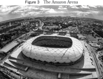
(6) . Figure 3 The Amazon Arena. Source: Portal da Copa, http://www.copa2014.gov.br/pt-br/galeria. of Manaus, the capital of the state of Amazonas, in the heart of Amazon Rainforest. The stadium is strategically situated between the international airport and the city’ s historic center. Architect Ralf Amann from the German firm GMP Architekten 4 authors the modern architectural project, inspired by the Amazon rainforest. Sustainability features include rainwater collection for reuse in the facilities’ restrooms and in watering the grass, natural ventilation to reduce energy costs, and solar energy production. It can receive up to 44,351 customers and accommodates over 400 cars in its underground parking lot. This year, it was elected the ninth top world stadium in 2014 according to the specialized British site“Stadium DataBase”5）. It was inaugurated on March 9, 2014 and hosted four of the 2014 World Cup games. Furthermore, it is expected to host several soccer matches of the Summer Olympic Games to be held in Rio de Janeiro in 2016. Because of its high cost of about 338 million US dollars6）and the unlikely use of its full capacity other than in very top-level competitions 7）, the construction of the Amazon Arena was heavily criticized as a“white elephant”during the street protest movement that took over the streets of Brazil in the months of June and July 2013 8）. Figure 3 presents a picture of the Arena. The Amazon Arena was chosen for two main reasons. First, it has a reasonably large number of items in its database (1724 items). Second, its has been carefully audited by the Brazilian Federal Court of Accounts (TCU), which allows us to compare the findings based on Benford’ s Law analysis with the results of TCU auditing. 4）http://www.gmp-architekten.com/projects. html. 5）http://stadiumdb.com/competitions/stadium_ of_the_year_2014. 6）According to Brazilian government of ficial data, its cost was R$ 632,841,524.06 (http://www. por taltransparencia.gov.br/copa2014/cidades/ execucoesFinanceirasDetalhe.seam;jsessionid=04F4 47F2E1BD0B12234EF627E923C033.por talcopa?exe cucaoFinanceira=13&empreendimento=5, accessed. June 6, 2015). We used the Febr uar y 15, 2010 Brazilian Central Bank Exchange rate. 7）According to Downie (2013),“The local teams who will use stadiums in the Amazon city of Manaus and Cuiaba in Brazil's western farm belt rarely get more than 1,000 fans at their games”. 8）For more infor mation on the 2013 street protests in Brazil and their relation with the World Cup expenditures, see The Economist (2013)..

(7) . 4. Tests of Benford’s law based on the digits’ frequencies. The tests used in the present study are carefully characterized in Nigrini (2012). This section presents their basic structure.. 4.1. First Digit Test According to NB Law, the expected relative frequency of a number in which the first digit D is d 1 is: 1. Table 1 presents these expected relative frequencies. Furthermore, Figure 4 plots these frequencies in a two dimensional graph. For the sake of illustration, Figure 4 also plots actual first digit relative frequencies for a database composed of Japanese cities’and Brazilian municipalities’populations in 2010. One striking empirical observation is that the proportions of first-digits 1 and 5 are exactly the expected ones for the Brazilian case. Furthermore, the relative frequencies of first-digits 4 and 7 are exactly the same for both populations’datasets, and both are very close to Benford’ s Law expectations. Table 1 Expected relative frequencies of first digits according to Benford’ s Law First digit Relative Frequency. 1. 2. 3. 4. 5. 6. 7. 8. 9. 30,10%. 17,61%. 12,49%. 9,69%. 7,92%. 6,69%. 5,80%. 5,12%. 4,58%. Source: Newcomb (1881). The test consists in comparing each digit’ s observed relative frequency with the predicted one by means of a typical Z-statistic. The Z-statistic is calculated as shown below, where i∊{1,2,3,4,5,6,7,8,9} is the analyzed first-digit category,. is the number of observations, RF is the actual relative frequency of. first-digit , and ERF is the expected relative frequency of first-digit .. The 5% significance level threshold is 1.96. If the Z-statistic of a first-digit exceeds 1.96, the frequency of the items starting with digit. does not conform to the predicted one. Therefore, that item is a. candidate for further scrutiny . 9）. 9）For the sake of illustration, only first-digit 2’ s Z-statistic exceeds the 1.96 threshold in the dataset consisting of Japanese populations whereas only first-digit 9 falls outside the compliance range for the Brazilian population dataset. This first result. suggests a reasonable conformity with Benford’ s Law..

(8) . Figure 4 Benford’ s Law predicted first digit relative frequencies and actual first digit frequencies in Japanese and Brazilian 2010 cities’ populations 0.350 0.300 0.250 0.200 0.150 0.100 0.050 0.000 1. 2. 3 Japan. 4. 5 Brazil. 6. 7. 8. 9. Benford. Source: Newcomb (1881), Local Administration Bureau, Japan Ministry of Internal Affairs and Communications and Brazilian Institute of Geography and Statistics, IBGE.. Nigrini (2012) suggests two criteria for overall compliance with MB Law based on the first-digit test. Firstly, a chi-square statistic is calculated as follows, where F is the actual frequency of first-digit and EF is its expected frequency according to Benford’ s Law.. The 5% confidence threshold critical value for 8 degrees of freedom is 15.507. Therefore, if the chi-square statistic exceeds 15.507 there is evidence of an overall non-conformity of the observed distribution with NB Law 10）. Finally, a mean absolute deviation (MAD) test is based on the absolute differences between observed and expected relative frequencies, according to the following statistic.. Nigrini (2012) proposes the following conformity criteria for the MAD test. If the MAD statistic is lower than 0.006, there is close conformity; if it is higher than 0.006 but lower than 0.012, there is acceptable conformity; if it lies in the interval (0.012, 0.015] there is marginally acceptable conformity and. finally, if it exceeds 0.015 there is nonconformity. 11）. 10）The high discrepancy for first-digits 2 for the case of Japan and 9 for the case of Brazil places both databases’ chi-square statistics above the conformity threshold. 11）The MAD statistics for the Japanese and. . the Brazilian populations are 0.0129 and 0.0053, respectively. This places the Japanese data in the lower part of the marginally acceptable conformity interval and the Brazilian one in the close conformity region..

(9) . Table 2 Expected relative frequencies of first two-digits according to Benford’ s Law (in percentage) First two digits Relative Frequency First two digits Relative Frequency First two digits Relative Frequency First two digits Relative Frequency First two digits Relative Frequency First two digits Relative Frequency First two digits Relative Frequency First two digits 8Relative Frequency First two digits Relative Frequency. 10. 11. 12. 13. 14. 15. 16. 17. 18. 19. 4.14. 3.78. 3.48. 3.22. 3.00. 2.80. 2.63. 2.48. 2.35. 2.23. 20. 21. 22. 23. 24. 25. 26. 27. 28. 29. 2.12. 2.02. 1.93. 1.85. 1.77. 1.70. 1.64. 1.58. 1.52. 1.47. 30. 31. 32. 33. 34. 35. 36. 37. 38. 39. 1.42. 1.38. 1.34. 1.30. 1.26. 1.22. 1.19. 1.16. 1.13. 1.10. 40. 41. 42. 43. 44. 45. 46. 47. 48. 49. 1.07. 1.05. 1.02. 1.00. 0.98. 0.95. 0.93. 0.91. 0.90. 0.88. 50. 51. 52. 53. 54. 55. 56. 57. 58. 59. 0.86. 0.84. 0.83. 0.81. 0.80. 0.78. 0.77. 0.76. 0.74. 0.73. 60. 61. 62. 63. 64. 65. 66. 67. 68. 69. 0.72. 0.71. 0.69. 0.68. 0.67. 0.66. 0.65. 0.64. 0.63. 0.62. 70. 71. 72. 73. 74. 75. 76. 77. 78. 79. 0.62. 0.61. 0.60. 0.59. 0.58. 0.58. 0.57. 0.56. 0.55. 0.55. 80. 81. 82. 83. 84. 85. 86. 87. 88. 89. 0.54. 0.53. 0.53. 0.52. 0.51. 0.51. 0.50. 0.50. 0.49. 0.49. 90. 91. 92. 93. 94. 95. 96. 97. 98. 99. 0.48. 0.47. 0.47. 0.46. 0.46. 0.45. 0.45. 0.45. 0.44. 0.44. Source: Nigrini (2012). 4.2. First-Two Digits Test According to NB Law, the expected relative frequency of a number in which the first digit, D 1, is. 1. and the second digit, D 2 , is d 2 is:. Table 2 presents these expected relative frequencies. Furthermore, Figure 5 plots these frequencies in a two dimensional graph. For the sake of illustration, Figure 5 also plots actual two-digits relative frequencies for the database composed of Japanese cities and Brazilian municipalities’populations in 2010. The figure highlights the striking non-conformity of two-digit 10 for the Brazilian database. Overall, the Japanese database appears to better conform to Benford’ s Law than the Brazilian one..

(10) . Figure 5 Benford’ s Law predicted first two-digits relative frequencies and actual first two-digit frequencies in Japanese and Brazilian 2010 cities’populations 0.070 0.060 0.050 0.040 0.030 0.020 0.010 0.000 10 13 16 19 22 25 28 31 34 37 40 43 46 49 52 55 58 61 64 67 70 73 76 79 82 85 88 91 94 97 Japan. Brazil. Benford. Source: Benford (1938), Local Administration Bureau, Japan Ministry of Internal Affairs and Communications and Brazilian Institute of Geography and Statistics, IBGE.. The test consists in comparing each two-digit’ s obser ved relative frequency with the (above) expected one by means of a typical Z-statistic. As in the first-digit case, the Z-statistic is calculated according to the formula below, where now i∊{10,11,…,99} is the analyzed two-digit category,. is the. number of observations, RF is the observed relative frequency of two-digits , and ERF is the expected relative frequency of two-digits .. The 5% significance level threshold is 1.96. If the Z-statistic of a two-digit exceeds 1.96, the frequencies of the items star ting with these two digits do not conform to the predicted ones. Therefore, these are the candidates for further inspection. Nigrini (2012) suggests three criteria for overall compliance with MB Law based on the two-digit tests. Firstly, if no more than 5 two-digits among all 90 classes {10,11,…,99} do not conform, there is no strong evidence of manipulation. Following up with the Japanese population example, the test found only 2 two-digit categories in the non-compliance range: 33 and 54. Therefore, there is overall conformance to Benford’ s Law. For the Brazilian database, on the other hand, there are 11 cases of non-compliance, which suggests that the data do not conform as closely to Benford’ s distribution. Secondly, a chi-square statistic is also calculated as follows, where F is the observed frequency of two-digits and EF is the expected frequency of two-digits ..

(11) . The 5% confidence threshold critical value for 89 degrees of freedom is 112.02. Therefore, if the chi-square statistic exceeds 112.02 there is evidence of an overall non-conformity of the observed distribution with NB Law. The Japanese population chi-square statistic is 72.56, confirming compliance with Benford’ s Law. However, the Brazilian chi-square statistic is 204.53, which does not conform to Benford’ s Law. Finally, a mean absolute deviation (MAD) test is based on the absolute differences between observed and expected relative frequencies, according to the following statistic.. Nigrini (2012) proposes the following conformity criteria for the MAD test. If the MAD statistic is lower than 0.0012, there is close conformity ; if it is higher than 0.0012 but lower than 0.0018, there is accept able conformity ; if it lies in the interval (0.0018, 0.0022] there is m argin ally accept able conformity. and finally, if it exceeds 0.0022 there is nonconformity . The corresponding figures for the Japanese and the Brazilian population databases are, respectively, 0.00178 and 0.00164, which places both databases in the range of acceptable conformity.. 4.3. Summation Test Nigrini (2012) simulated a Benford distribution and separated the resulting sample into 90 classes according to the first two digits {10,11,…,99}. Then, he added all number observations in each group and found evidence that all sums led to approximately the same amounts. In other words, the numbers in each class tended to sum up to 1/90=0.011 or 1.1% of the total sum of all numbers in the sample. However, the author found that actual data rarely conformed completely to such a standard. The usefulness of this test is precisely to point out the nonconformities. Whenever the sum of values in one category represents a too high percentage of total summation in the database, then there is room for doubting of the authenticity of the values in that category. There are no threshold explicitly suggested by Nigrini (2012); therefore, we consider here a difference higher that 100% of the expected 1.1% percentage to be the upper bound for conformity in our analysis. In other words, a realized percentage above 2.2% or, equivalently, a difference higher than 1.1%=0.011 will be considered an evidence of manipulation.. 4.4. The confrontation between the two tests Any two-digit category that falls into the nonconformity criteria range for either the Z-test or the summation test is a candidate for further scrutiny. However, some two-digit categories may fall into nonconformity simply because of their lack of frequency in the database. In that case, it might be an unrewarding task to dedicate time analyzing the corresponding items. Therefore, we propose to.

(12) . compare the frequencies of all categories that have been selected in at least one of the two tests. If one of them shows very little frequency according to both criteria, i.e., there are few observations in that category and the value of the summation of the category’ s items is low, then that category should be excluded from further scrutiny. We call this comparison the“confrontation”of the two tests. Our main point in doing the confrontation is that, in the case of public works’budget, the pecuniary relevance of each group should be taken into account for selecting the digits that need further auditing. 5. Analysis of Amazon Soccer arena’s construction procurement. 5.1 The Amazon Arena’s construction budget worksheet The analysis of this study focused on the budget of Amazon soccer arena’ s constr uction originally presented to TCU by the procurement winning firm in the amount of R$ 615,992,824.67 (US$329,937,214.36 as of February 15, 2010 12）). Subsequently, after the TCU auditing, alternative budgets that aimed at eliminating detected overpricing of most worksheet items were negotiated. We selected the initial budget for three main reasons. First, the subsequent budgets were changed after the TCU auditing; therefore, these budget sheets were not entirely formulated by the winning bidder. Since we wish to detect possible data manipulation from that bidder, the original bid should be used. Second, the first budget sheets were subject to careful TCU auditing that revealed significant overpricing. Therefore, we will be able to compare the results of our analysis based of NB Law with the results of TCU’ s auditing. Third, the TCU analysis is based on the ABC cur ve methodology, which consists of ordering the items in a budget sheet from most expensive to least expensive and selecting up to 20% of the most expensive items, until the total cost of those items adds up to about 80% of the total budget, and them compare those prices with market benchmarks. Therefore, the TCU did not make use of our proposed methodology in its analysis, which makes the comparison valuable. The budget worksheet contains both each individual item’ s cost and the corresponding total cost, which consists of the quantity of an item multiplied by the unit cost of that item. For the sake of application of NB Law we could use either the unit costs or the total costs data in our database. In another application (The Maracanã Soccer Arena, see Cunha and Bugarin, 2015) we used the unit costs and our analysis was able to detect 71.54% of total overprice uncovered by the TCU auditing. Considering that Benford’ s Law is more likely to apply to databases which elements come from the multiplication of different random variables, such as account receivable or budget worksheets (quantities times unit prices/costs, see, for instance, Cho and Gaines, 2007), we decided to use the total costs database. . The database consists of 1724 items; all the corresponding total costs had at. 13）. least two digits. Therefore, all data was used in our analysis.. 12）A c c o r d i n g t o B r a z i l i a n C e n t r a l B a n k US$1.00=R$1.867 on Februar y 15, 2010. From here on we will use that exchange rate for all calculations without further mention. We chose that date for the calculations of the dollar amounts because this is the. time the TCU performed its audit on the winning bid’ s budget worksheets. 13）We also performed the analysis based on unit costs, which yielded similar results. The details are available upon request..

(13) . Table 3 The First Digits Relative Frequencies First digit Sample relative frequency Benford's Law relative frequency. 1. 2. 3. 4. 5. 6. 7. 8. 9. 0.313. 0.208. 0.103. 0.083. 0.076. 0.058. 0.053. 0.054. 0.052. 0.301. 0.176. 0.125. 0.097. 0.079. 0.067. 0.058. 0.051. 0.046. Source: Newcomb (1881) and authors’calculations. Figure 6 Benford’ s Law predicted first digit relative frequencies and actual first digit frequencies in Amazon Arena budget worksheet 0.350 0.300 0.250 0.200 0.150 0.100 0.050 0.000 1. 2. 3. 4. 5. 6. 7. 8. 9. Actual relative frequencies Benford's Law expected relative frequencies Source: Newcomb (1881) and authors’calculations. 5.2. First Digit Test The first-digit’ s relative frequencies are reported in Table 3. Figure 6 presents the corresponding graph and compares is with the expected relative frequencies according to Benford’ s Law. The results of the first digit tests are reported in Table 4, where:“Digit”refers to the first digit; “Frequency”is the absolute frequency (count) of items staring with the corresponding first digit in the worksheet;“Actual”is the corresponding relative frequency;“NB”is the expected relative frequency according to NB Law;“Diff”is the difference between“Actual”and“NB”;“Z-Test”refers to the Z-statistic;“CS”is the Chi-Square statistic intermediate calculation; and“MAD”is the Mean Absolute Deviation statistic intermediate calculation. The Chi-Square statistic is the sum of column“CS” whereas the MAD statistic is the sum of column“MAD”. The Z-test indicates abnormal frequencies for the digits 2 and 3, with 2 appearing too frequently whereas there is abnormally low frequency of first digit 3. This suggests most especially careful auditing of items whose total costs have first digit 2. The chi-square statistic is the sum of all intermediate values in column CS: 25.639. The critical value for 8 degrees of freedom and 5% significance level is 15.507. Therefore, we reject the null hypothesis, suggesting non-conformity with NB Law. Finally, the MAD test-statistic is the mean of the sum of all intermediate values in column MAD: 0.0118, which suggests acceptable conformity according to the criterion adopted by Nigrini (2012)..

(14) . Table 4 First Digit Tests for total costs of Amazon Arena soccer stadium Digit 1 2 3 4 5 6 7 8 9. Frequency. Actual. NB. Diff.. Z-Test. CS. MAD. 540 359 178 143 131 100 91 93 89. 0.313 0.208 0.103 0.083 0.076 0.058 0.053 0.054 0.052. 0.301 0.176 0.125 0.097 0.079 0.067 0.058 0.051 0.046. 0.012 0.032 -0.022 -0.014 -0.003 -0.009 -0.005 0.003 0.006. 1.080. 0.856 10.179 6.526 3.510 0.198 2.082 0.809 0.293 1.185. 0.012 0.032 0.022 0.014 0.003 0.009 0.005 0.003 0.006. 3.483 2.694. 1.931 0.419 1.446 0.875 0.501 1.057. N = 1724 observations calculations Source: Authors’. To summarize, the tests based on the first digit may suggest possible manipulation of data. Auditing based only on the first digit test, however, may be a long and fruitless task. Indeed, according to our data, over 20% of the total number of observations has first digit 2. Therefore, only those items would already fill the usual number of audited items TCU uses in its ABC curve approach. Furthermore, due to the high level of aggregation (the database is partitioned in only 9 groups), there may be additional items in other categories in which manipulations cancel out within a category. For these reasons, additional analysis is in order.. 5.3. First-Two Digits Test The results of the first-two digits tests are reported in Table 5, where, as before:“Digit”refers to the first two digits;“Frequency”is the absolute frequency of items staring with the corresponding first two-digits in the worksheet;“Actual”is the corresponding relative frequency;“NB”is the expected relative frequency according to NB Law;“Diff”is the difference between“Actual”and“NB”;“Z-Test” refers to the Z-statistic;“CS”is the Chi-Square statistic intermediate calculation; and“MAD”is the Mean Absolute Deviation statistic intermediate calculation. Figure 7 plots the actual two digits relative frequencies against the ones predicted by Benford’ s Law..

(15) . Table 5 First-Two Digits Tests for total costs of Amazon Arena soccer stadium Digit 10 11 12 13 14 15 16 17 18 19 20 21 22 23 24 25 26 27 28 29 30 31 32 33 34 35 36 37 38 39 40 41 42 43 44 45 46 47 48 49 50 51 52 53 54. Frequency. Actual. NB. Diff.. 45 82 67 43 64 52 55 53 55 24 37 26 39 31 36 29 16 77 30 38 18 30 12 20 21 23 13 17 12 12 25 18 16 12 8 16 11 20 7 10 18 10 15 12 11. 0.026 0.048 0.039 0.025 0.037 0.030 0.032 0.031 0.032 0.014 0.021 0.015 0.023 0.018 0.021 0.017 0.009 0.045 0.017 0.022 0.010 0.017 0.007 0.012 0.012 0.013 0.008 0.010 0.007 0.007 0.015 0.010 0.009 0.007 0.005 0.009 0.006 0.012 0.004 0.006 0.010 0.006 0.009 0.007 0.006. 0.041 0.038 0.035 0.032 0.030 0.028 0.026 0.025 0.023 0.022 0.021 0.020 0.019 0.018 0.018 0.017 0.016 0.016 0.015 0.015 0.014 0.014 0.013 0.013 0.013 0.012 0.012 0.012 0.011 0.011 0.011 0.010 0.010 0.010 0.010 0.010 0.009 0.009 0.009 0.009 0.009 0.008 0.008 0.008 0.008. -0.015 0.010 0.004 -0.007 0.007 0.002 0.006 0.006 0.008 -0.008 0.000 -0.005 0.003 -0.001 0.003 0.000 -0.007 0.029 0.002 0.007 -0.004 0.004 -0.006 -0.001 0.000 0.001 -0.004 -0.002 -0.004 -0.004 0.004 0.000 -0.001 -0.003 -0.005 0.000 -0.003 0.002 -0.005 -0.003 0.002 -0.003 0.000 -0.001 -0.002. Z-Test 3.127 2.065. 0.864 1.636 1.673 0.464 1.370 1.502. 2.230 2.269. -0.005 1.426 0.913 0.065 0.901 -0.025 2.230 9.518. 0.634. 2.423. 1.230 1.183. 2.211. 0.394 0.044 0.308 1.558 0.555 1.585 1.491 1.406 -0.108 0.268 1.142 2.040. -0.011 1.152 0.946 2.029. 1.195 0.697 1.064 0.063 0.401 0.606. CS. MAD. 9.738 4.359 0.834 2.810 2.949 0.280 2.034 2.433 5.207 5.403 0.006 2.239 0.982 0.024 0.967 0.005 5.317 90.973 0.528 6.272 1.748 1.632 5.290 0.247 0.023 0.173 2.752 0.441 2.853 2.553 2.294 0.000 0.149 1.579 4.630 0.013 1.617 1.139 4.612 1.737 0.679 1.417 0.038 0.284 0.546. 0.015 0.010 0.004 0.007 0.007 0.002 0.006 0.006 0.008 0.008 0.000 0.005 0.003 0.001 0.003 0.000 0.007 0.029 0.002 0.007 0.004 0.004 0.006 0.001 0.000 0.001 0.004 0.002 0.004 0.004 0.004 0.000 0.001 0.003 0.005 0.000 0.003 0.002 0.005 0.003 0.002 0.003 0.000 0.001 0.002.

(16) . Digit 55 56 57 58 59 60 61 62 63 64 65 66 67 68 69 70 71 72 73 74 75 76 77 78 79 80 81 82 83 84 85 86 87 88 89 90 91 92 93 94 95 96 97 98 99. Frequency. Actual. NB. Diff.. Z-Test. CS. MAD. 6 15 16 17 11 5 9 9 8 7 9 5 10 28 10 3 6 7 14 9 10 8 16 11 7 6 4 9 5 13 6 6 9 20 15 14 6 9 10 13 9 15 4 5 4. 0.003 0.009 0.009 0.010 0.006 0.003 0.005 0.005 0.005 0.004 0.005 0.003 0.006 0.016 0.006 0.002 0.003 0.004 0.008 0.005 0.006 0.005 0.009 0.006 0.004 0.003 0.002 0.005 0.003 0.008 0.003 0.003 0.005 0.012 0.009 0.008 0.003 0.005 0.006 0.008 0.005 0.009 0.002 0.003 0.002. 0.008 0.008 0.008 0.007 0.007 0.007 0.007 0.007 0.007 0.007 0.007 0.007 0.006 0.006 0.006 0.006 0.006 0.006 0.006 0.006 0.006 0.006 0.006 0.006 0.005 0.005 0.005 0.005 0.005 0.005 0.005 0.005 0.005 0.005 0.005 0.005 0.005 0.005 0.005 0.005 0.005 0.005 0.004 0.004 0.004. -0.004 0.001 0.002 0.002 -0.001 -0.004 -0.002 -0.002 -0.002 -0.003 -0.001 -0.004 -0.001 0.010 0.000 -0.004 -0.003 -0.002 0.002 -0.001 0.000 -0.001 0.004 0.001 -0.001 -0.002 -0.003 0.000 -0.002 0.002 -0.002 -0.002 0.000 0.007 0.004 0.003 -0.001 0.001 0.001 0.003 0.001 0.004 -0.002 -0.002 -0.002. 1.911 0.344 0.689 1.038 0.307. 4.159 0.231 0.681 1.379 0.199 4.396 0.828 0.741 1.219 1.829 0.517 3.480 0.108 26.657 0.055 5.468 1.910 1.072 1.427 0.110 0.001 0.326 4.159 0.224 0.621 1.172 2.929 0.001 1.755 1.934 0.868 0.815 0.023 15.740 5.261 3.964 0.582 0.101 0.496 3.253 0.172 6.758 1.763 0.890 1.651. 0.004 0.001 0.002 0.002 0.001 0.004 0.002 0.002 0.002 0.003 0.001 0.004 0.001 0.010 0.000 0.004 0.003 0.002 0.002 0.001 0.000 0.001 0.004 0.001 0.001 0.002 0.003 0.000 0.002 0.002 0.002 0.002 0.000 0.007 0.004 0.003 0.001 0.001 0.001 0.003 0.001 0.004 0.002 0.002 0.002. Number of observations 1724 Source: authors’calculations. 1.962. 0.769 0.719 0.962 1.210 0.573 1.722 0.178. 5.028. 0.083. 2.192. 1.231 0.882 1.041 0.174 -0.133 0.413 1.884 0.312 0.627 0.921 1.550 -0.141 1.161 1.226 0.765 0.735 -0.020 3.805 2.126. 1.822 0.590 0.143 0.529 1.630 0.236. 2.426. 1.150 0.764 1.105.

(17) . Figure 7 Benford’ s Law predicted first-two digit relative frequencies and actual first-two digit frequencies in Amazon Arena budget worksheet 0.060. 0.050. 0.040. 0.030. 0.020. 0.010. 0.000 10 13 16 19 22 25 28 31 34 37 40 43 46 49 52 55 58 61 64 67 70 73 76 79 82 85 88 91 94 97 Actual. Benford. Upper Bound. Lower Bound. Number of observations: 1724, the Upper bound and Lower bound curves refer to the 95% significance level Source: Authors’calculations. According to Table 5, there is evidence of non-conformity in the digits 10, 11, 18, 19, 26, 27, 29, 32, 44, 48, 60, 68, 70, 88, 89 and 96 with respect to the proportions of the descending curve of NB Law. These corresponds to 16 two-digit categories exceeding the limit of 1.96, a number very much above the threshold of 5 peaks suggested by Nigrini (2012). Therefore, the Z-test suggests that the data have been manipulated. It is noteworthy that some of the peaks correspond to numbers that appear too frequently whereas others correspond to numbers that appear too seldom. Naturally, we would expect that the ones that appear too frequently are the top candidates for being manipulated data. In particular, one should stress first-two digits 27 and 68 (see Figure 7). The Chi-Square statistic, the summation of column CS, is 293.736. The critical value for 89 degrees of freedom and 5% significance level is 112.02. Therefore, we reject the null hypothesis, suggesting, again, non-compliance with NB Law. The last test applied is MAD. The test statistic found for Amazon Arena is 0.0033, which highly exceeds the 0.0022 threshold adopted by Nigrini (2012). This result suggests, once again, possible manipulation of data.. 5.4. Summation Test In order to assess the pecuniar y significance of each pair of digits in the budget worksheet we perform the complementary Summation Test. The results are shown in Table 6 below, where the 1st.

(18) . column refers to the first-two digits of the observations; the 2nd column corresponds to the sum of the total costs of items that have the first-two digits indicated in the 1st column; the 3rd column shows the proportions of the sums calculated in the 2nd column with respect to the total costs of the worksheet; and column 4 computes the difference between the actual proportions of the sums and the expected ones. Recall that the expected proportions of each sum of total cost in each two-digit category is 1.1% or 0.011, according to Nigrini (2012). Recall, furthermore, that we have set an upper bound threshold of 0.022 for conformity. Therefore, Table 6 highlights peaks in the first two digits 11, 12, 13, 14, 15, 52, 60, 67, 77 and 78. It is noteworthy the very high ratio of appearance of two-digits 60, representing 20.7% of total costs. The test strongly suggests nonconformity to NB Law..

(19) . Table 6 Summation Test for total costs of Amazon Arena soccer stadium Digit 10 11 12 13 14 15 16 17 18 19 20 21 22 23 24 25 26 27 28 29 30 31 32 33 34 35 36 37 38 39 40 41 42 43 44 45 46 47 48 49 50 51 52 53 54. Sum. Actual. Benford. 6,779,337.27 13,321,384.80 16,925,818.66 19,373,384.39 22,580,106.79 28,505,937.80 8,798,956.04 5,324,811.18 5,174,192.59 9,160,737.42 5,700,596.87 5,706,353.64 4,128,765.13 7,594,421.93 10,850,773.13 6,773,131.14 3,718,898.40 9,754,202.70 1,467,372.18 5,378,772.64 6,774,856.16 5,134,543.48 1,114,827.30 581,314.36 5,699,104.65 5,754,647.32 1,568,419.89 1,370,164.55 220,564.72 756,380.76 9,925,971.95 10,243,159.92 1,170,449.44 1,530,502.13 1,071,595.82 601,959.44 1,506,748.31 1,714,607.67 6,377,647.71 227,670.25 1,226,073.95 698,252.58 53,463,119.57 7,026,444.91 355,504.46. 0.011 0.022 0.027 0.031 0.037 0.046 0.014 0.009 0.008 0.015 0.009 0.009 0.007 0.012 0.018 0.011 0.006 0.016 0.002 0.009 0.011 0.008 0.002 0.001 0.009 0.009 0.003 0.002 0.000 0.001 0.016 0.017 0.002 0.002 0.002 0.001 0.002 0.003 0.010 0.000 0.002 0.001 0.087 0.011 0.001. 0.011 0.011 0.011 0.011 0.011 0.011 0.011 0.011 0.011 0.011 0.011 0.011 0.011 0.011 0.011 0.011 0.011 0.011 0.011 0.011 0.011 0.011 0.011 0.011 0.011 0.011 0.011 0.011 0.011 0.011 0.011 0.011 0.011 0.011 0.011 0.011 0.011 0.011 0.011 0.011 0.011 0.011 0.011 0.011 0.011. Difference. 0.000. 0.011 0.016 0.020 0.026 0.035. 0.003 -0.002 -0.003 0.004 -0.002 -0.002 -0.004 0.001 0.007 0.000 -0.005 0.005 -0.009 -0.002 0.000 -0.003 -0.009 -0.010 -0.002 -0.002 -0.008 -0.009 -0.011 -0.010 0.005 0.006 -0.009 -0.009 -0.009 -0.010 -0.009 -0.008 -0.001 -0.011 -0.009 -0.010 0.076. 0.000 -0.010.

(20) . Digit 55 56 57 58 59 60 61 62 63 64 65 66 67 68 69 70 71 72 73 74 75 76 77 78 79 80 81 82 83 84 85 86 87 88 89 90 91 92 93 94 95 96 97 98 99. Sum. Actual. Benford. Difference. 734,563.64 942,726.17 1,990,461.73 2,000,276.50 7,540,247.05 127,223,393.04 332,069.66 948,407.85 783,863.39 329,013.41 2,122,060.55 332,589.49 9,486,088.97 315,803.31 854,916.40 78,632.23 8,697,745.38 313,056.63 2,611,687.45 7,655,137.69 279,397.79 329,847.91 78,725,633.04 17,555,153.59 414,123.69 185,950.12 913,013.16 133,992.08 343,503.97 2,848,420.58 351,228.64 185,162.72 2,041,493.74 407,834.26 2,018,837.03 1,255,957.83 2,030,709.91 999,639.96 2,107,473.07 1,354,079.96 1,095,960.57 1,613,890.82 39,068.09 306,419.34 30,806.34. 0.001 0.002 0.003 0.003 0.012 0.207 0.001 0.002 0.001 0.001 0.003 0.001 0.015 0.001 0.001 0.000 0.014 0.001 0.004 0.012 0.000 0.001 0.128 0.028 0.001 0.000 0.001 0.000 0.001 0.005 0.001 0.000 0.003 0.001 0.003 0.002 0.003 0.002 0.003 0.002 0.002 0.003 0.000 0.000 0.000. 0.011 0.011 0.011 0.011 0.011 0.011 0.011 0.011 0.011 0.011 0.011 0.011 0.011 0.011 0.011 0.011 0.011 0.011 0.011 0.011 0.011 0.011 0.011 0.011 0.011 0.011 0.011 0.011 0.011 0.011 0.011 0.011 0.011 0.011 0.011 0.011 0.011 0.011 0.011 0.011 0.011 0.011 0.011 0.011 0.011. -0.010 -0.009 -0.008 -0.008 0.001. Number of observations: 1724 Source: Authors’ calculations. 0.196. -0.010 -0.009 -0.010 -0.010 -0.008 -0.010 0.004 -0.010 -0.010 -0.011 0.003 -0.010 -0.007 0.001 -0.011 -0.010 0.117 0.017. -0.010 -0.011 -0.010 -0.011 -0.010 -0.006 -0.010 -0.011 -0.008 -0.010 -0.008 -0.009 -0.008 -0.009 -0.008 -0.009 -0.009 -0.008 -0.011 -0.011 -0.011.

(21) . Table 7 Confrontation between the First-Two Digits Test and Summation Test Digits 10 11 12 13 14 15 18 19 26 27 29 32 44 48 52 60 68 70 77 78 88 89 96. First-Two Digits Test 0.026 0.048 0.039 0.025 0.037 0.030 0.032 0.014 0.009 0.045 0.022 0.007 0.005 0.004 0.009 0.003 0.016 0.002 0.009 0.006 0.012 0.009 0.009. Benford. Summation Test. Critical Digits. 0.041 0.038 0.035 0.032 0.030 0.028 0.023 0.022 0.016 0.016 0.015 0.013 0.010 0.009 0.008 0.007 0.006 0.006 0.006 0.006 0.005 0.005 0.005. 0.011 0.022 0.027 0.031 0.037 0.046 0.008 0.015 0.006 0.016 0.009 0.002 0.002 0.010 0.087 0.207 0.001 0.000 0.128 0.028 0.001 0.003 0.003. No Yes Yes Yes Yes Yes Yes No No Yes Yes No No No Yes Yes Yes No Yes Yes Yes Yes Yes. Source: author’ s calculations. 5.5. Confrontation between the First-Two Digits Test and the Summation Test Next, we select the digits detected as critical in the First-Two Digits Test and Summation Test. Then we carr y out a confrontation between these tests to confirm the sample relevance of the selected digits, comparing their relative frequency in each one of the tests. All two digits that show low relative frequency in both tests correspond to items that do not appear frequently in the database and, furthermore, to item which aggregate costs are not very significant as percentage of total budget. Therefore, these two-digit items are considered non-critical points: it is not worthy to spend the auditors’time analyzing these items. Table 7 shows the digits that were selected by either one of the tests in column 1. Column 2 shows the relative frequencies of these digits according to the first-two digit tests. Column 3 displays the proportions of the sum of total costs of items starting with these digits according to the Summation test. Column 4 singles out the two-digits that have little significance in the spreadsheet according to both criteria: low percentage of items starting with those two digits and low sum of the corresponding values as percentage of the sum of all items (No). The confrontation between the tests suggests excluding digits 10, 19, 26, 32, 44, 48, 68, 70 and 88 from our analysis. Therefore, our methodology suggests the following critical points for the auditing process: 11, 12, 13, 14, 15, 18, 27, 29, 52, 60, 77, 78, 88, 89 and 96..

(22) . 6. Comparison with the Brazilian Court of Accounts’ analysis. Brazilian TCU performed a careful analysis of the initial winning bidder’ s budget sheet, requiring a series of price and quantity adjustments in order to approve the contract. We will compare TCU findings after the analysis of that initial winning bidder’ s budget sheet with our analysis based on Benford’ s Law. Table A1 in the Appendix presents the output of TCU’ s audit. This audit compared the winning bid’ s budget sheets with market prices as of February 2010. Therefore, all figures presented here in dollars use the exchange rate of February 15, 2010 according to the Brazilian Central Bank. To perform that comparison a few details on the TCU methodology is in order. As we explained earlier, the TCU uses the ABC curve methodology, which consists of ordering the items according to their total costs in decreasing order, and audit up to 20% of all such ordered items, starting from the most expensive to the least expensive ones, until the total cost of those items adds up to 80% of the total budget. In the present case the TCU analysis total audited items’costs amounted to R$492,594,332.98 (US$263,842,687) out of a total budget of R$615,992,824.67 (US$329,937,214.36), which corresponds to 79.97% of the entire budget. The TCU introduced two types of aggregation when ordering the items. (i) First, due to the complexity of the project, some items were repeated several times in the worksheet. Each time, the item referred to a different part/stage of the construction. The unit price was always the same, naturally, but the quantities change according to the expected use. Therefore, the same item appeared with different codes and total prices throughout the budget worksheet. For example, the item“Ferragens de aço CA-50A”(Steel hardware of type CA-50A) appeared under 19 different item codes, corresponding to total costs in 15 two-digit categories. . The TCU’ s analysis. 14）. output aggregates all observations of the same item in the budget sheet and analyses it as one item. (ii) Second, the TCU performs two types of analysis for each item: price and quantity. In other words, the TCU analyses if the total quantity proposed in the worksheet is adequate and also if the unit price reflects market prices. (iii) Third, in some cases the TCU found actually that the total cost of an item has been undercalculated by the bidder, usually because the market prices determined by TCU are higher than what appeared in the worksheet. In that case, a negative number appears in the TCU overprice estimation. Therefore, TCU’ s overprice estimate corresponds to the net amount resulting of the substraction of total underprices from the total overprice. (iv) Fourth, the TCU found it difficult to analyze the cost of air conditioning services. Therefore, it aggregated all items related to air conditioning, calculated their total cost in the budget worksheet, then calculated the total amount of refrigeration to be generated by the system (in tons of refrigeration, TR) and then divided the total cost by the total amount of refrigeration (652 TR) in order to obtain the per-unit-of-refrigeration cost. This was used to calculate overprice in that category, which amounted to R$2,613,808.35 (US$1,400,004.37). 14）The two-digit categories are: 10, 11, 12, 13, 16, 19, 20, 23, 24 (three different codes), 25, 34, 42, 59, 65, 67, 78 and 94..

(23) . Table 8 Confrontation between the results of tests of the NB Law and TCU’ s overpricing analysis for the digits 11, 12, 13, 14, 15, 18, 27, 29, 60, 77, 78 and 89, in Brazilian Reals as of February 2010 Digit. Item code. Overpricing detected by TCU. 11.4.1 11. 12. 13. 14. 15. 18 27. 29. (in Brazilian Real, R$). 6,235,225.71. 15.105. 13,555.84. 24.10. 202,334.75. 24.26. 78,798.00. 24.34. 5,859,425.46. 8.17. 338,948.36. 8.11 (Already uncovered). 6,235,225.71. 24.31 (Already uncovered). 5,859,425.46. 8.12. 6,249,520.46. 11.4.2 (Already uncovered). 5,859,425.46. 24.27 (Already uncovered). 6,235,225.71. 13.15. 124,310.17. 13.19. 706,545.34. 24.15. 1,993,872.00. 7.1. 610,038.38. 10.5. 1,253,793.13. 13.2. 504,835.29. 15.108. 758,675.38. 11.7.2 (Already uncovered). 5,859,425.46. 15.51. 431,398.36. 11.8.5. 6,387,800.00. 14.1. 1,141,339.79. 11.6.2(Already uncovered). 5,859,425.46. 8.6. 145,951.68. 24.5 (Already uncovered). 202,334.75. 24.12 (Already uncovered). 78,798.00. 52. 12.3. 8,827,023.45. 60. 4.2. 22,180,663.27. 77. 24.21 (Already uncovered). 78,798.00. 6.16. 5,915,199.94. 78 89. 9.10 (Already uncovered). 1,993,872.00. 11.2.1 (Already uncovered). 6,235,225.71. 24.1. 443,855.34. Total Source: Brazilian Court of Accounts, TCU and authors’ calculations. 70,403,110.10.

(24) . Given the above explanations, we performed our comparison as follows: (i) Each observation of a repeated item with overprice detected by TCU placed that item in a (possibly different) two-digit category. If any one of these categories was signaled out by our Benford’ s Law tests, then we say that the item has been uncovered by our methodology, and compute the total overprice determined by TCU. (ii) What matters to our analysis is the manipulation of worksheet total values, be it by manipulating quantities or prices. Therefore, since we are analyzing total costs, it is irrelevant to us where the manipulation came from. (iii) Since we aim at uncovering overprices, we did not subtract underprice uncovered by TCU. Therefore, for our analysis, the total overprice uncovered by TCU was used, corresponding to a total amount of R$90,394,830.23 (US$48,417,152.41). This is higher than the amount that appears in TCU’ s audit output (Table A1, Appendix), which is R$86,544,009.11. (iv) Finally, there is no way our analysis can incorporate the aggregation of all different items that compose the air-conditioning system. Therefore, we will not be able to uncover the corresponding overprice (R$2,613,808.35) detected by TCU. If one subtract that amount from total overprice (R$90,394,830.23) then we obtain T=R$87,781,021.88 (US$47,017,148.04). T is the upper bound for whatever the methodology we propose, based on Benford’ s Law, can possibly uncover of overprices. We use T as the reference for our comparison. Table 8 presents the comparison with the TCU analysis. TCU’ s ABC Cur ve analysis identified overpricing in several items that had one of these critical digits as the first two digits of the total costs; the total overpricing for these ser vices was R$ 70,403,110.10 (US$37,709,215.27) as of February 2010. This corresponds to 80.20 % of total overpricing (R$87,781,021.88 or US$47,017,148.04) uncovered by TCU. It is very important to stress that TCU auditors work on a very tight time schedule. Therefore, the better the selection of data to be analyzed, the better the result of their analysis. The ABC curve is a rather efficient and standard methodology based on selecting the most expensive items. The methodology we propose, based on Benford’ s Law, suggests a different ordering of data. In the present application, if all the two-digit categories that our methodology suggests were audited, this would amount to only R$402,021,662, which corresponds to only 65.26% of the total budget. In spite of the reduced budget auditing sample, our methodology would have allowed us to single out 80.20% of total overpricing found by TCU. It is noteworthy that TCU did note audit all items in the categories we suggest. We might only wonder if additional overprices would not have found if a complete audit of all two-digits highlighted by the methodology based on Benford’ s Law had been performed. Note, moreover, that had we chose a lighter criterion for the summation test, more two-digit would have been singled out, increasing the performance of the auditing process. This suggests the algorithmic approach that we present in next section. 7. Proposition: An algorithm for selecting the auditing sample. Based on the previous considerations, we now propose an algorithm for determining the sample to be audited. There are five main parameters..

(25) . Figure 8 An algorithm based on Benford’ s Law to select the audit sample Step Step 1:. Action. Setting up the initial values. Set ＝80%, ＝5%, ＝100%, ＝25%, ＝5%. Set T ＝the total cost of the budget.. Step 2:. Set Below＝false. Two-digit test.. Step 3:. Apply the two-digit test using the significance criterion Select the corresponding two digit categories. Summation test. If. Step 4:. Step 5: Step 6:. .. ＞ 10% then set Below＝true and go to Step 7.. If ≤ 0 then set = ＋5%, set = + and go to Step 2. Apply the summation test with the threshold, i.e., select all two-digit categories with relative frequency above 0.011( 1＋ ) in the summation calculation. Confrontation between the two-digit and the summation tests Perform the confrontation between the two-digit test and the summation test to select the auditing sample, A . Auditing budget cost. Calculate the total cost of the sample in the budget worksheet, S . Compare the sample and the entire worksheet costs. Compute. Step 7:. If. then go to Step 7.. If. and S ＜T then set. ＝ −. and go to Step 3.. If and S ＞T then set ＝＋ and go to Step 3. Audit sample S. If Below＝false, then we were able to select a sample with total cost near the target of B . If Below＝true, the methodology based on Benford’ s Law was unable to signal out a number of two-digit categories high enough so that the corresponding cost nears the target of B .. Source: Authors’proposal. The parameter. reflects the percentage of the total budget cost to be audited. It is set here at. 80% in order to preserve the present standard used in the ABC curve methodology, as explained earlier; however, other standards could also be used. The parameter reflects the significance level to be used in the two-digit test. Following Nigrini (2012), it is initially set at 5%. reflects the initial threshold to be used in the summation test. Following our The parameter proposal, it is initially set at 100%. The parameter reflects the adjustment to be made to the summation test significance level parameter , as will become clear in what follows. It is set here at 25%. Finally, the parameter reflects the precision of the stop criterion, i.e., how close the total cost of.

(26) . the selected sample is from the targeted percentage. of total budget. We set this parameter at. 5%. The main goal of the algorithm is to select a sample that contains the observations that are most likely to have been manipulated according to the tests inspired in Benford’ s Law, while auditing about. (percent) of the total cost of the budget worksheet, whenever possible. Figure 8 details the. algorithm. The main idea behind the algorithm is to start with the basic parameters and select the first audit sample. If that audit sample’ s total cost is already near the target 80% of the budget’ s total cost, then that is the final sample. If it’ s total cost is too large, then straighten the selection criterion of the summation test to reduce the sample size. If the cost is too low, then relax the selection criterion of the summation test to augment the sample size. If it is not possible to augment the sample size by relaxing the summation test criterion anymore, but the sample total cost is still too low, then relax the confidence level of the two-digit test to 10%. No more relaxations are allowed. If the final sample’ s total cost is still too low, then the algorithm was not able to select enough items based exclusively on Benford’ s Law criteria. In that case, the sample may be completed with other criteria, such as the cost of items, as in the ABC curve methodology. This final completion is not introduced here. For the sake of illustration, let us apply the algorithm to the Amazon Arena worksheet. The first iteration allows us to select the two-digit categories are: 11, 12, 13, 14, 15, 18, 27, 29, 52, 60, 77, 78, 88, 89 and 96. The corresponding sample total cost is: S ＝R$402,021,662 and it corresponds to 65.26% of total costs. This is the analysis we already performed in section 4. The second iteration reduces the upper bound threshold for the summation test from 0.022 to 0.0195, but no new two-digit category is added. The third iteration reduces the upper bound threshold for the summation test to 0. 0165 and allows us to add the two-digit categories 24 and 41. The corresponding sample total cost is: S ＝R$423,115,595 and it corresponds to 68.69% of total costs. The fourth iteration reduces the upper bound threshold for the summation test to 0. 01375 and allows us to add the two-digit categories 16, 19, 40 and 67. The corresponding sample total cost is: S ＝ R$460,487,349 and it corresponds to 74.76% of total costs. The fifth iteration suggests reducing the two-digit test significance level to 10%, rather than 5%. Although three new categories are selected according to the two-digit test (55, 66 and 90), none of these categories pass the confrontation with the summation test and the algorithm concludes with Below＝true, i.e., we were not able to detect additional categories to audit based on Benford’ s Law. The final auditing sample suggested by this methodology is. S ＝{11,12,13,14,15,16,18, 19,24,27,. 29,40,41,52,60,67,77,78,88,89,96}. The total cost of items in that sample is S ＝R$460,487,349 and it corresponds to 74.76% of total costs. Note that many of the items in sample S where not audited by TCU. Therefore, it is not possible to assert whether that sample, were it indeed audited, would lead to findings of overprice not detected by the traditional ABC curve. However, we can observe that our methodology was able to uncover 81.65% of total overprice found in the TCU audit..

(27) . 8. Conclusion. The present research tested the application of Newcomb-Benford’ s Law to the total costs of the budget worksheet for the construction of Amazon Arena soccer stadium. The main goal of the methodology is to point to which items might be more likely to have been manipulated, thereby might correspond to overestimated costs. It applied the First Digit Tests, First-Two Digits Test and the Summation Test, all based of Benford's Law, using the Z-statistic, the Chi-Square and the Mean Absolute Deviation tests. All tests point to a non-conformity of the database to Benford’ s Law, which suggests that the costs presented in the budget worksheets may have been manipulated. Next, our analysis singled out thirteen first-two-digit categories of total prices 11, 12, 13, 14, 15, 18, 27, 29, 52, 60, 77, 78 and 89 which contained items that were shown by TCU analysis to have been overpriced by a total amount of R$ 70,403,110.10 (US$37,709,215.27) as of Febr uar y 2010, which corresponds to over 80% of total overprice uncovered by TCU. In particular, that analysis was able to uncover the single item with highest overprice, item 4.2, in the two-digit categor y 60, with overprice of R$22,180,663.27 (US$11,880,375.80). Comparing the total cost associated to the actually audited sample with the sample suggested by our methodology, we find out that it corresponds to about 65% of the entire procurement cost, whereas the TCU audited about 80% of it, as established by the ABC curve’ s methodology. To conclude, our paper proposes an algorithm to select the sample to be audited in an alternative, possibly more efficient fashion, while still auditing about 80% of total procurement cost. To be certain, more empirical work is needed in order to fully compare the two methodologies. For example, two teams could perform simultaneously the auditing, one using the Benford’ s Law derived methodology and a second one using the traditional ABC curve and the results could be compared ex-post. Naturally, for the sake of the res publica, the two teams would have to aggregate their findings once the auditing would be concluded. This additional robustness test is left here as a suggestion for future research. It is noteworthy to discuss the possible future of data manipulation in government procurements. Indeed, at least in the case of Brazil, Newcomb-Benford’ s Law has not yet being applied as a regular, complementar y tool by the Brazilian Cour t of Accounts, which, in par t, may explain the highly significant result found in the present analysis. However, if this tool becomes standard, bidding firms might become aware of it and may devise more sophisticated ways to overprice their bids in order to try avoiding detection. However, as we tried to illustrate by the complementary use of the first digit, two-digits and the summation tests, Benford’ s Law is a very rich tool and several diverse tests may be applied to a single database. For example, there is also a simple test for the second digit. Whereas it may be a feasible task to manipulate data while keeping the expected relative frequencies for the first digits, it may be a much harder task to keep data in conformity to the expected relative frequencies of the first two digits, the second digit, and the summation. Therefore, the authors do not anticipate simple manipulation algorithms in the near future. Furthermore, additional tests are been developed everyday, and new laws can alternatively be used, such as the Zipf’ s Law (Odueke & Weir, 2012), which is, in a specific way, a generalization of Benford’ s Law. Recent trends towards increased globalization requires developing countries’government to invest heavily in expensive large-scale infrastructure projects in order to keep on the map of an ever more.

(28) . competitive world. In a context of capital constraint, it is essential to keep public procurement works at their lowest possible cost while ensuring the required quality of the final output. Benford’ s Law has been successfully used to test data manipulation in very diverse areas, from accounting and financial data to tax returns, macroeconomic and electoral data. The present work illustrates the successful use of the Law as a tool to help auditors of large public work projects and suggest that Benford Law should be regularly used in the public auditor’ s toolbox. References. Benford, F. (1938)“The law of anomalous numbers" . Proceedings of the American Philosophical Society 78 (4), 551-572. Berton, L. (1995)“He’ s got their number: scholar uses math to foil financial fraud”. Wall Street Journal. 10, B1, July 10.. Cho, W. T. and B. Gaines (2007)“Breaking the (Benford) Law: Statistical Fraud Detection in Campaign Finance”. The American Statistician 61(3): 218-223. Cunha, F. R. da and M. Bugarin (2015)“Benford’ s Law for audit of public works: an analysis of overpricing in Maracanã soccer arena’ s renovation”. Economics Bulletin 35 (2): 1168-1176. Downie, A. (2013)“Brazil protests pose challenge for World Cup organisers”. Reuters , June 19, 2013. Available at <http://in.reuters.com/ar ticle/2013/06/18/brazil-protests-socceridINDEE95H0FW20130618>. Accessed June 6, 2015. Durstchi, C., W. Hillison and C. Pacini (2004)“The ef fective use of Benford’ s Law to assist in detecting fraud in accounting data”. Journal of Forensic Accounting V: 17-34. Economist, The (2013)“Protests in Brazil – The streets erupt”. The Economist , June 18, 2013. Available at < http://www.economist.com/blogs/americasview/2013/06/protests-brazil>. Accessed June 6, 2015. European Commission (2010)“Report on Greek Government Deficit and Debt Statistics”. Available at <http://epp.eurostat.ec.europa.eu/portal/page/portal/product_details/publication? p_product_ code=COM_2010_report_greek>. Accessed on July 10, 2014. Hill, T.P. (1995)“Base-Invariance Implies Benford's Law”. Proc. Amer. Math. Soc . 123, 887-895. Mebane, W. R. (2006)“Election Forensics: vote counts and Benford’ s Law”. Summer Meeting of the Political Methodology Society. Papers, Posters and Syllabi. Nº 620. ______ (2010)“Fraud in the 2009 presidential election in Iran?”Chance 23(1), 6-15. ______ (2009)“Note on the presidential election In Iran”. Updated notes on author’ s website. Available at http://www.benfordonline.net/fullreference/756. Accessed July 10, 2014. Newcomb, S. (1881)“Note on the frequency of the different digits in natural numbers”. The American Journal of Mathematics 4(1), 39-40.. Nigrini, M. J. (1992) The Detection of Income T ax Evasion Through an Analysis of Digital Frequencies . Ph.D. thesis. Cincinnati, OH: University of Cincinnati. ______ (2000) Digital analysis using Benford’s L aw: Tests Statistics for Auditors . Global Audit Publications: Vancouver. _____ (2012) Benford’s L aw. Applications for Forensic Accounting Auditing, and Fraud Detection . John Wiley & Sons, Inc.: Hoboken, New Jersey..

(29) . Odueke, A., and G. Weir (2012)“Triage in Forensic Accounting using Zipf’ s Law”in: Weir, G. and A. Al-Nemrat, Issues in Cybercrime, Security and Digtal Forensics . University of Strathclyde Publishing, 33-43. Rauch, B., G. Brähler and M. Göttsche (2011)“Fact and Fiction in EU-Governmental Economic Data”. German Economic Review 12(3), 243-255.. Appendix. The Brazilian Federal Court of Accounts audit of Amazon Arena 2014 World Cup soccer stadium We present the result of TCU’ s audit in Table A1. Note that TCU aggregated several observation of one same item that appeared at different moments in the winning bid worksheet. We added the right-most column to make clear how to make the two-digit comparison. The original detailed budget worksheet sheet is available upon request to the authors. The first column of Table A1 describes the items. For the sake of simplicity and space we kept the original description in Portuguese and dropped part of it when the descriptions were too long. In that case we replace the final part of a description with the symbol […]. The line in a different color corresponds to the bundled items related to air conditioning. Because different items where bundled together for analysis, we could not apply Benford’ s Law the bundled items. Note that some items were not audited. These corresponded to the following two-digit categories: 14, 18, 19, 20, 30 and 31. Had our methodology been followed, the items corresponding to the to-digit categories 14, 15 and 18 would have been audited. Their combined budget was: R$4,916,251.58 (US$2,633,235.79)..

(30) . Table A1 The Brazilian Federal Court of Accounts Audit of Amazon Arena 2014 World Cup soccer stadium, February 2010 ACTIVITY (ITEM). UNIT. Cobertura em balanço com malha de vigas de aço intertravadas [...]. Executive project budget Qunatity. Unit price. KG. 3,510,000.00. 22.00. Fachada em malhas "x" de vigas intertravadas para revestimento [...]. KG. 2,749,000.00. 22.00. Administração local - projeto executivo. URAL. 36.00. Membrana têxtil em fibra de vidro PTFE. M2. 31,000.00. Ferragem de aço Ca-50 a. KG. 5,108,143.68. Total price. Final overprice. Two-digit category. 77,224,674.84 3,510,000.00. 22.00. 77,224,674.84. 0.00. 77. 60,481,661.29 2,842,720.00. 22.00. 62,539,840.00. -2,058,178.71. 60. 37,950,153.48 22,180,663.27. 60. 43,348,146.55. 8,827,023.45. 52. 6,235,225.71. 10, 11, 12, 13, 16, 19, 20, 23, 24 (three different codes), 25, 34, 42, 59, 65, 67, 78 and 94.. 5,859,425.46. 41, 40 (two different codes), 35, 27, 24, 23, 22, 15, 13, 12, 11 and 10. 1,670,300.47 60,130,816.75 1,683.07. 8.32. TCU audit Unit price. Total price. 52,175,170.00. Quantity. 36.00. 1,054,170.93. 31,000.00. 1,398.33. 42,474,214.69 4,971,054.73. 7.29. Concreto fck 40 mpa alto desempenho (CAD) com adição de microssílica e fibra de polipropileno. M3. 30,847.21. Assento retrátil geral. UN. 40,761.00. Projeto executivo. CJ. 1.00. Concreto especial estaca hélice fck 20 mpa autoadensável. M3. 17,626.32. 810.42. 14,284,722.25. 12,292.82. 653.65. Forma plana aparente chapa compensada plastificada de 18 mm, com [...]. M2. 139,441.17. 91.08. 12,700,301.77. 139,441.17. Serviços agrupados do sistema de ar condicionado (excluindo os dutos). TR. 652.00. 13,365.95. 8,714,596.22. Concreto prémoldado fck 40 mpa alto desempenho [...]. M3. 7,378.56. 1,389.28. Concreto fck=35 mpa. M3. 10,373.80. Demolição mecanizada de estrutura de concreto armado, exceto pisos [...]. M3. Transportes projeto executivo TRANSPORTE, LANÇAMENTO E ESPALHAMENTO DE MATERIAL ESCAVADO [...]. 816.80. 25,196,001.14. 30,847.21. 383.69. 15,639,588.09. 40,554.00. 36,238,988.98. 626.85. 19,336,575.68. 373.20. 15,134,752.80. 504,835.29. 15. 15,450,000.00 15,450,000.00. -626,559.15. 14. 8,035,201.79. 6,249,520.46. 13 and 63. 45.27. 6,312,501.77. 6,387,800.00. 30, 27, 22, 21, 16 and 90. 652.00. 9,357.04. 6,100,787.87. 2,613,808.35. -. 10,250,885.84. 6,925.45. 1,182.39. 8,188,582.83. 2,062,303.01. 48 and 53. 785.82. 8,161,718.53. 10,373.80. 594.56. 6,167,846.53. 1,993,872.00. 14, 16 and 78. 23,846.83. 327.53. 7,810,552.23. 23,846.83. 79.48. 1,895,352.29. 5,915,199.94. 78. MÊS. 36.00. 205,763.26. 7,407,477.36. 36.00. 190,511.39. 6,858,409.99. 549,067.37. 74. M3. 325,934.00. 21.85. 7,121,657.90. 325,934.00. 18.69. 6,093,153.19. 1,028,504.71. 71. 14,823,440.85 14,823,440.85. 1.00.