札幌における宇宙線強度の観測 (英文)
10
0
0
全文
(2) Vol. 10, No. 1 Journal of Hokkaido Gakugei University July, 1959. Observation of Cosmic-Ray Intensity at Sapporo. Motoo YOSHIDA, Eitaro KOMIYA, Yoshihiro SEGAVVA. and Yoshihiro NAKANO. Physics Laboratory, Hokkaido Gakugei University, Sapporo. ^BTT:^, ^j^^^p, djnx^, ^'sf-^^: ^if%{c:^y-^^mi^^®i. Some aspects of the continuous observation of cosmic-ray intensity in the period of I. G. Y. using "Nishina" type ionization chamber are described. Variations of cosmic-ray intensity and their relations to several meteorological factors are also examined.. § 1. Introduction Though not a few stations have been performing the continuous observation of cosmicray intensity all around the world up to now, the scale of the station net work was expanded in the I. G. Y. started in July, 1957. In Japan, hitherto, only three stations were operating as cosmic-ray observatories; two of them are in Tokyo (Itabashi and Mabashi) and the other is at Mt. Norikura. However, they are at the almost same position in the geomagnetic latitude (about 25° Nm). At these circumstances, our physics laboratory started the continuous. observation in the earlier stage in 1957 at Sapporo, which is sited at the highest geomagnetic latitude in Japan (about 33° Nm). Now, our laboratory is designated as one of the cosmic-ray observing stations in the world by the C. S. A. G. I. The cosmic-ray data of the continuous observation at Sapporo have been obtained from April, 1957 and sent to the I. G. Y. Data Center ever since the I. G. Y. started. These full data are published from the I. G. Y. Data Center. Using our data during this interval, the variations of cosmic-ray intensities and their relations to several meteorological factors were examined. § 2. Apparatus and I. G. Y. Data The measurements have been carried out on the top of our university building at Sapporo. (longitude 141° 21/ E, latitude 43° 02/ N, magnetic latitude 32° 55/ N,n and height 54 m above sea level). The apparatus is the "Nishina" type ionization chamber of which the detail is described in our previous report1-1. The chamber is shielded by lead of 10cm thick and. set in a thermally regulated box (at 28°C,). The data are obtained from the photographic film recording the voltage variations of electrometer needle, which is turned to zero potential automatically every one hour. The mean cosmic-ray intensity is compensated by the ionization. from the uranium source which is plugged in the chamber and gives the voltage variation rate of 7.846 mV/sec. The relative ratios of the bihourly values of cosmic-ray intensity with the mean value are obtained in the unit of 0.1%. These values are described as I (bihourly intensities uncorrected) and after the correction of barometric pressure effect with the coefficient ^-=— 0.11%,.
(3) M. Yoshida, E. Komiya, Y. Segawa and Y. Nakano. mb, it is denoted as Ip. The time of bihourly value is given in the scale of Universal Time U. T. (Greenwich IVIean Time). The data at Sapporo in the following are being sent every month to the I. G. Y. Data Center. i) Uncorreeted bihourly values / of cosmic-ray intensity obtained by our ionization chamber. ii) Corrected value Ip by the barometric effect based on the effective correction coefficient ^——0.11%/mb and the mean barometric pressure at Sapporo as 1010mb. iii) Barometric pressure P at Sapporo after reduction to sea level value.. iv) Height H and temperature T at several isobaric levels (1000 mb, 700 mb, 500 mb, 300 mb, 200 mb, 100 mb and 50 mb) at Sapporo obtained from the radio-sonde flying every day at 09 and 21 o'clock in local time.. These P, H and T data are supplied by Sapporo Meteorological Observatory (northern about 2 km apart from our laboratory). The full data will be published by the I. G. Y. Data Center soon, so the each tables are not given here.. § 3. Atmospheric Effect Cosmic-ray arriving at the bottom of atmosphere already suffered the absorption by air mass and the cosmic-ray mesons are decaying through the length of path in the atmospheric gases. So the observed intensities at ground are varied with the meteorological conditions. To get the true knowledge for the primary cosmic-ray, it must be corrected accordingly. In the I. G. Y. report the barometric correction coefficient is taken as 0.11%/mb from other recommendation^. In this paper, these meteorogical correction coefficients are checked in each seasons.. These coefficients are tried statistically under the assumption of linear relations. In the calculations, the daily mean values used are sellected under the following conditions. i) The day has more than eleven bihourly values in /. ii) The period does not involve the remarkable magnetic or solar disturbances. iii) The day does not miss so much meteorological data.. Calculations are carried out with their effective days given by Table I in each period. Table I. Period. I. II. m. IV. v. VI. Season. Spring. Summer. Autum. Winter. Spring. full year. 1-5-57. 9-7-57. 4-10-57. 3-12-57. 8-3-58. 1-5-57. to. 31-5-57. 21-9-57. 20-11-57. 26-2-58. 28-6-58. 26-3-58. eft", days. 30. 43. 30. 60. from. 60. 173. 3-1. Barometric pressure eflEect. The relationship between the I and P is very clear when plotted in the same time sequence. It is found at first that they are at negative correlation as are shown in our previous paper0. If we consider only a single correlation, the correlation coefficient is found to be fairly large, almost -0.7~-0.8 for each season, and that is nearly constant. However, even if we introduce the other meteorological factors (such as H or T} and take double.
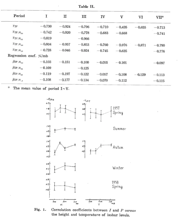
(4) Observation of Cosmic-Ray Intensity at Sapporo Table II.. I. II. Ill. IV. v. VI. VIP. rip. -0.730. -0.924. -0.796. -0.710. -0.435. -0.655. -0.713. rrp."3». -0.742. -0.920. -0.778. -0.683. -0.668. ^I'.H.B. -0.819. rip.H,,. -0.804. -0.957. -0.853. -0.760. -0.976. HP.HIO. -0.728. -0.946. -0.924. 0.745. -0.635. -0.776. -0.151. -0.100. -0.055. -0.101. -0.097. Period. -0.741. -0.966. -0.871. -0.790. Regression coef. ^/mb <3IP."30. -0.103. <3lP,H^. -0.109. 0IP.H.O. -0.119. -0.197. -0.122. -0.057. -0.108. (9 IP,H^. -0.108. -0.177. -0.134. -0.070. -0.112. -0.125 -0.129. -0.113. -0.115. The mean value of period I~V.. -^IP-H 0.-^). 19V?. 11. Sprmg. Simme r. AzituTTl. I ~i. Winter. 19%. Spr'lTi^. Fig. 1. Correlation coefficients between I and P versus. the height and temperature of isobar levels. correlations, the correlation coefficients are practically unchanged. These values are shown. in Table II and Fig. 1. Taking the averages of the regression coefficients in seasons and other meteorological factors, the value is determined as —0.112% /mb, which is in good agreement with the already accepted values as correction coefficients. Accordingly, the correction coefficient (3=— 0.11%, mb is considered to be useful for our data. But, when this value is examined carefully, it. is noticed that systematic deviations are left behind, this point will be discussed in the following section..
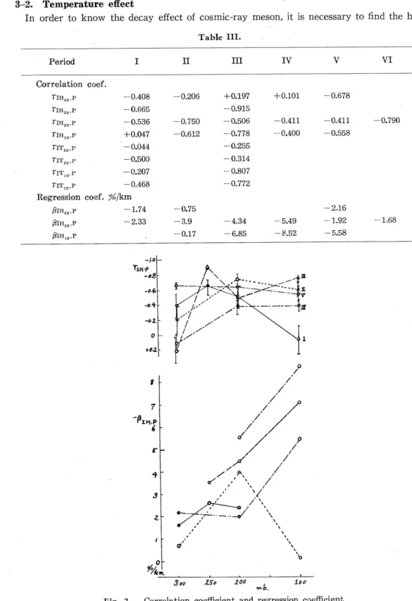
(5) M. Yoshida, E. K.omiya, Y. Segawa and Y. Nakano. 3-2. Temperature effect In order to know the decay effect of cosmic-ray meson, it is necessary to find the height Table III.. II. Period. m. IV. v. +0.197. +0.101. -0.678. VI. Correlation coef. T-IH^.P. -0,408. riH,,.p. -0.665. -0.206. -0.915. rm^.p. -0.536. -0.750. -0.506. -0.411. -0.411. ^lH»o.P. +0.047. -0.612. -0.778. -0.400. -0.558. rix^.v. -0.044. -0.255. n'i\,,f. -0.500. -0.314. rrr^.p. -0.207. -0.807. riT,,.p. -0.468. -0.772. Regression coef.. ^/km. -2.16. ^IHso.P. -1.74. -0.75. 0IH,,.P. -2.33. -3.9. -4.34. -5.49. -1.92. -0.17. -6.85. -8.52. -5.58. 0IH,o.P. -/.oh-. riH-P. -e8\ -0^. \ .^..-.. ^--~/^<^-~-^-<..\. -0.^ -ll-t\. 0 *OA|. ./. .7. 7 '^Xh.P. </ r. 4. ^. 0^. /. /. /. /" / '/,. ^.\. y. J. /. /. /. ./. /. /N'. z. ^a. -0.790. 3 co ^So. 2.00. -k. loo. Fig. 2. Correlation coefficient and regression coefficient between I and H refering to sea level pressure.. 4 -. -l.e.
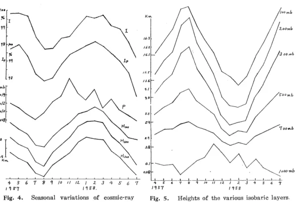
(6) Observation of Gosmic-Ray Intensity at Sapporo of meson production level, but this level is not determined uniquely. It is only shown that nearly the 100 mb atmospheric layer has the most remarkable effect as production layer. Partial correlations between the cosmic-ray intensity and the heighs or temperatures of. isobaric levels (100 mb, 200 mb, 250 mb and 300 mb) in the condition of the constant barometric pressure at ground are examined. Those partial correlation coefficients and effective coefficients over seasons are given in Table III and Fig. 2. Though these values are not so large to have strong significance, the correlation with the height of 200 mb level is the most remarkable in every season. If we have determined the correction coefficient for temperature effect, it will become more favourable to use the. 200 mb level height. But to determine the correction coefficient is impossible, for our data are not yet full enough in the present stage. §4, Time and seasonal variations in cosmic-ray intensity Cosmic-ray intensity and meteorological circumstances are changing time to time. It varies in one side as statistical fluctuations, and in the other periodically. The periods are classified in some ways, such as daily, monthly, yearly and over several years, so the cosmic-ray intensities suffer time and seasonal variations. Our data are not so sufficient enough. ^%. to discuss these effect completely, that, here,. +0.2.. " \'. only diurnal and seasonal effect are discu&sed. 40.;. 4-1. Mean diurnal variation All the Ip values are arranged hour to hour and the results are given in Fig. 3, also with atmospheric pressure data P. The curve shows. -1-t I. '-^. 0. /p' \-t. -0.1. a maximum at 14 o'clock and minimum at 4 o'clock in local time, and the amplifcude of the variation is 0.17%, This result is in good agreement with those from other authors3'1. Pressure curve shows a half day period and. -OA 1111. 1111...... I. I. I. I. 8 lo li ,4 16 IS 20 2JL SA- ^o A,e»^ ti-^e.. Fig. 3. Diurnal variation of cosmic-ray. a minimum at 14 o'clock in local time; however,. intensities (Ip) and barometric pressure (P) (1-4-1957-31-3-1958). the amplitude is smaller.. In the other hand, it is expected that the mass of air is displaced upward at about 14 o'clock due to solar heating, and this is important in connection with meson decay in the effect of reducing the cosmic-ray intensity at sea level, so we can expect a minimum to occur at this time. But, on the contrary with this expectation, we have a maximum nearly at the time. This may be regarded as the contribution of the particles coming from the Sun entering into the earth near the noontime. 4-2. Seasonal effect In order to find the relationship between the seasonal variations of the cosmic-ray intensity and the meteorological factors, these data are arranged month to month in Figs. 4, 5 and 6. As is shown in Fig. 4, all curves have similar tendency. I and Ip show minima in August and maxima in February. P curves are showing minima in summer and maxima in winter,. but the seasonal variations are very small. The height of 200 mb isobaric level plotted in inverse phase is very similar to the Ip curve, then the seasonal variations in cosmic-ray. intensity are influenced mostly by the height of this level, 5—.
(7) M. Yoshida, E. Komiya, Y. Segawa and Y. Nakano. 67?'?/o///Z/2J4^-67. •|^S€^a•:tl<'lll^l2.3^So'f. ns-s.. Fig. 4. Seasonal variations of cosmic-ray pig. 5. Heights of the various isobaric layers. intensity and other several meteorological factors,. -I". -S-o|. -4»| -r»l -1"\ -JO -JO. -3.1. -I". 45- 6 78 <i 10 n n i i 3 ^ 5 & ^ I. IS-7.. I. IS. 8.. Fig. 6. Temperatures of the isobaric layers.. 6—.
(8) Observation of Cosmic-Ray Intensity at Sapporo The heights and temperatures of the, 100 mb,. -VlP.H. 200 mb and etc. isobaric levels are given in Figs. 5 and 6 respectively. In the former, we see the. ».°1. same behavior of variations, that is, maxima in. »-1\. summer (July~August) and minima in winter. oS[. (January~March). The temperature of 200 mb. 0.1\. level is almost constant throughout the year,. 6&\. above and below this level it alters in the opposite direction.. 300 mb. a) Correction coefficient of pressure. ———100 mb. Pressure correction coefficients calculated in. .—- I 00 mb. -/4P.H. each season are given in Table II and are plotted. in Fig. 7. The following will be noticed; these. 0.2,1-. coefficients are the largest in summer and the smallest in winter, medium values in spring and autumn, and the recurrency is rather good. This seasonal effect may be caused by the miscellaneous atmospheric conditions determining the. ^. o.\. pressure at ground which is different in each season. This effect is recognized in the data of other stations'0'5-'.. y^>. b) Temperature effect Temperature correction coefficients given in. m. Table III have not any seasonal effects as are plotted in fig. 2. The points are so widely dispersed that the meaningful results can not be. Peripei Fig. 7.. found.. TV. Correlation coefficients (T'n'.n) and regression coefficients (/3ip.n) refering to the seasonal period.. c) Diurnal variation Bihourly values are calculated hour to hour every month and are compared among them.. The methods of finding diurnal variation in every month are the following; 1) Amplitude is the difference of a certain' mean value from the daily mean. The former mean is determined by the six bihourly values larger than the latter daily mean.. 2) Intensity maximum time is determined as the center of the six bihourly points at which they are larger in the intensity than the mean value, and this centeral time is called as the phase of variation. Plotting polar vector diagram using these amplitudes and phases, it is shown in Fig. 8 that the maximum time is changing almost every half a year. In winter and spring, the phase is at about 15 o'clock, in summer and autumn at about 13 o'clock in local time, and the amplitude is the largest in summer. § 5. Bursts In the ionization chamber, the elecrometer needle is moving continuously at normal condition, but occasionally when heavy ionizations occur in the chamber, then the needle suddenly jumps, and these phenomena are called as bursts. In our apparatus, the minimum burst which can be read from our recording film corresponds to about 2x10 ionpairs/min,.
(9) M. Yoshida, E. Komiya, Y. Segawa and Y. Nakano. flS-7. /»•. \. \. A.. \. fo. 0.3.^.. ,0. Fig. 8. Phase diagram of diurnal. I -\. -^L—J—i,. /o If Jt» Tiy,. Fig. 9. Burst size versus frequency. variations of cosmic-ray. (1-4-57~31-5-58).. intensities in each month.. (this value means the larger ionization than the normal intensity by a factor 3 or 4). These bursts are explained in two ways as are following; the first is that when heavy particles collides with the chamber wall, then many electrons are ejected and originate heavy ionizations, and the second is that multiple particle tracks, say, air shower core, provoke heavy ionization on the whole. Therefore, the bursts are high energy events, its frequency is considered as the number of high energy particles or events, and the size is proportional to the incident particle energy. Ferquency vs. size curve in this research period is drawn in Fig. 9, this is a energy-frequency spectrum, whose slope gives the index of power law spectrum, that is, E~1-8, which is consistent with the known values. § 6. Conclusion and Acknowledgements As is described in this paper, the continuous observation of cosmic-ray intensity at our laboratory is almost running smoothly. Some meteorological correlation factors are determined, and the reliability of our data are checked to be rather good. In the new period of I. G. C. following the I. G. Y., we should like to express our sincere thanks to Dr. Y. Miyazaki and the members of Cosmic-Ray Laboratory of Physico-Chemical Research Institute for their continuous helps and encouragements. ,.
(10) Observation of Gosmic-Ray Intensity at Sapporo. References. 1) Y. Nakano, M. Yoshida, Y. Ssgawa and E. Komiya : Journal of Hokkaido Gakugei University (Section B) Vol. 8, No. 1 (1957) p. 12 (in Japanese). 2) This value is used in the analysis of the ionization chamber data at I. P. C. R. 3) U. Pasoli and J. Pohl-Ruling : Nuovo Gimento, Vol. VI, No, 6 (1957) 1338. 4) F. Bachelet and A. M. Conforto : Nuovo Cimento, Vol. IV, No. 6 (1956) 1479. 5) M. Wada : Report of Cosmic-ray Laboratory of I. P. C. R,, Vol. 2, No. 1 (1953) 306 (in Japanese).. 9.
(11)
図

+3


関連したドキュメント
The purpose of this paper is analyze a phase-field model for which the solid fraction is explicitly functionally dependent of both the phase-field variable and the temperature
We have formulated and discussed our main results for scalar equations where the solutions remain of a single sign. This restriction has enabled us to achieve sharp results on
Keywords: continuous time random walk, Brownian motion, collision time, skew Young tableaux, tandem queue.. AMS 2000 Subject Classification: Primary:
Kilbas; Conditions of the existence of a classical solution of a Cauchy type problem for the diffusion equation with the Riemann-Liouville partial derivative, Differential Equations,
The oscillations of the diffusion coefficient along the edges of a metric graph induce internal singularities in the global system which, together with the high complexity of
In this work we give definitions of the notions of superior limit and inferior limit of a real distribution of n variables at a point of its domain and study some properties of
The study of the eigenvalue problem when the nonlinear term is placed in the equation, that is when one considers a quasilinear problem of the form −∆ p u = λ|u| p−2 u with
Then it follows immediately from a suitable version of “Hensel’s Lemma” [cf., e.g., the argument of [4], Lemma 2.1] that S may be obtained, as the notation suggests, as the m A
