Estimating long-term uplift rate based on
stream analysis:A practical guide to extract
tectonic signature from river morphology
著者
Takahashi Naoya
学位授与機関
Tohoku University
博士論文
Estimating long-term uplift rate based on stream analysis:
A practical guide to extract tectonic signature from river
morphology
(河川形状解析による長期的隆起速度推定と
実用化に向けた指針)
Naoya TAKAHASHI
令和2年
Abstract
Fault slip rate reflects sizes and recurrence intervals of past earthquakes, meaning
quantifying slip rates is vital to understand the spatiotemporal pattern of large earthquakes. Traditional approaches to obtain slip rates require offset markers that record deformation of past earthquakes; however, such marker is very limited. River adjusts its morphology depending on uplift rates and occurs ubiquitously, suggesting river morphology can be an alternative proxy to infer uplift rates. While a growing number of studies examine relationships between river morphology and uplift rates, we do not know how to use the current knowledge to derive more accurate uplift rates from stream analysis. Therefore, this thesis aims to provide a guide to tease out tectonic signals from river morphology through the following two studies.
In the first study, I presented a method to evaluate the effects of substrate strength on channel steepness based on the standard detachment limited model. Although the significance of substrate properties over channel morphology has long been recognized, the erosional resistance of rocks measured by existing methods was qualitative. The current method can quantify and calibrate the effects of different substrates on channel steepness. Using this method, I estimated the long-term uplift rates along the Futagawa fault, a dextral-normal fault in Kumamoto, southwestern Japan. Although further studies are necessary to test the robustness of this approach, the calibration method presented in this study should help evaluating effects of rock strength on normalized channel steepness.
The second study revealed the response timescales of channel width and hillslope angle to accelerated erosion. Channel width and hillslope angle are important factors to modulate erosion rates. Their response timescales were rarely discussed in previous studies due to their difficulty in
constraining in an actual landscape. I showed those response time could be constrained using knickpoint travel time and the resulting timescales were 320–540 ky for width and 40–320 ky for hillslope angle when the slope exponent n in the stream power model was 1. This result indicates that a basin-scale steady state is not established soon after a knickpoint travels up to the head of the trunk stream, emphasizing the need to carefully investigate trunk and tributary channels and adjacent hillslopes to reduce errors in uplift rates deduced from stream analysis.
Acknowledgment
First of all, I would like to show gratitude to my advisor, Shinji Toda, for his continuous encouragement and guidance since I entered this graduate school. He always let me do whatever I want and offered me countless opportunities to interact with other researchers, work in the field, attend conferences, and apply for research grants. I can never forget that we walked so hard in the steep mountains during the surface rupture mapping in Kumamoto, which inspired me very much and prepared me to work hard in the field. If he was not my advisor, my Ph.D. life and future career path would have been entirely different.
I would also like to thank Bruce Shyu for kindly accepting the offer to be my co-advisor and giving me tremendous support. Without his guidance on stream analysis, I could not have written this thesis. I cannot thank him enough for allowing me to stay in his lab, providing opportunities to meet many people who enriched my daily and research life in Taiwan.
I am grateful to all the staff of the International Joint Graduate Program In Earth and Environmental Sciences for allowing me to study abroad, offering financial support, and organizing exciting workshops and seminars. In particular, I want to thank Shin Ozawa and Shinobu Okuyama for their continuous and kind support.
I would like to thank the faculty members of the department of Earthscience and at
International Research Institute of Disaster Science in Tohoku University for providing administrative supports, comments on my work, and a comfortable research environment.
I owe analysis of 10Be to people at Disaster Prevention Research Institute (DPRI), Kyoto University. Yuki Matsushi kindly agreed to start a collaboration, gave me financial support, and allowed me to conduct experiments at DPRI. Ryoga Ohta spent a great deal of time to teach me the dating method and help me interpret the result. Akiko Morikawa taught me the experiment. Kazuko Kitamura arranged my stay at DPRI.
I have been fortunate to meet many people who provided comments on my work at seminars and conferences. Especially, I would like to thank Chia-Yu Chen for teaching me how to use
Topotoolbox and discussing the results, and Daisuke Ishimura for always being ready to discuss anything and giving me many opportunities to work in the field.
the biggest challenge in my life, and I could not have survived the last three years without having you around. Yasushi Itoh and Yongsheng Huang were always happy to talk over anything. Chi-Hsien Tang helped me stay sane when writing this thesis. Sze-Chieh Liu, Yu-Hsuan Yin, Cheng-Hung Cheng, and many other Taiwanese friends helped my life in Taiwan in many aspects.
Lastly, I would like to express my sincere gratitude to my parents. In any situation, they respected my decisions and provided continuous support for me. Although I have no idea when I can find a secure job, their presence makes me feel reassured and helps me pursue my interests.
Contents
CH. 1. INTRODUCTION ________________________________________________ 1
1.1.BACKGROUND ... 1
1.2.OBJECTIVE AND OVERVIEW ... 3
CH.2. CALIBRATING EFFECTS OF ROCK STRENGTH ON CHANNEL
STEEPNESS TO INFER ROCK UPLIFT __________________________________ 6
2.1.INTRODUCTION ... 62.2.STUDY AREA... 8
2.2.1. Tectonic setting ... 8
2.2.2. Substrate rock types ... 10
2.2.3. Basin characteristics ... 11
2.3.METHODS ... 13
2.3.1. Longitudinal river profile and channel steepness ... 13
2.3.2. Calibrating rock erodibility ... 14
2.3.3. Channel width measurement ... 15
2.4.RESULTS ... 16
2.4.1. ksnalong the Futagawa fault and the Idenokuchi fault ... 16
2.4.2. ksn dependency on substrate rock types ... 20
2.4.3. Channel width dependency on lithology ... 26
2.5.DISCUSSION ... 26
2.5.1. Channel width ... 29
2.5.2. Precipitation ... 29
2.5.3. Erosion process... 29
2.5.4. Implications for long-term relative uplift and earthquake recurrence ... 33
2.5.5. Limitation of our approach ... 34
2.6.CONCLUSIONS ... 35
CH. 3. RESPONSE TIMESCALES OF CHANNEL WIDTH AND HILLSLOPE
ANGLES TO ACCELERATED INCISION ESTIMATED FROM A KNICKPOINT
TRAVEL TIME ________________________________________________________ 36
3.1.INTRODUCTION ... 36
3.2.STUDY AREA... 38
3.3.METHODS ... 42
3.3.1. Observation of channel and hillslope morphology ... 42
3.3.2. Basin-averaged erosion rate determined from cosmogenic 10Be concentration ... 46
3.3.3. Knickpoint migration speed and response timescales ... 49
3.4.RESULTS ... 51
3.5.DISCUSSION ... 76
3.5.1. Implications for a basin-scale response timescale ... 76
3.5.2. Implications for better constraints on erosion and uplift rates... 81
3.6.CONCLUSION ... 82
CH. 4. CONCLUSION _________________________________________________ 83
4.1.SUMMARY AND RESEARCH NEEDS ... 834.2.CONCLUSION ... 85
REFERENCE _________________________________________________________ 86
SUPPLEMENTARY MATERIAL __________________________________________ I
List of Figures
Fig. 1.1. Evolution of a fault scarp
Fig. 1.2. A schematic illustration of river response to an increase in uplift rates Fig. 2.1. Topography and geology of the study area
Fig. 2.2. Comparison of channel width measured in the field and using 0.5m DEM
Fig. 2.3. Long-term uplift rates and vertical displacement of the Kumamoto earthquake along the Futagawa and the Idenokuchi fault
Fig. 2.4. Normalized channel steepness for trunk streams flowing across the Futagawa and the Idenokuchi fault
Fig. 2.5. Normalized channel steepness for trunk streams flowing across the Hinagu fault
Fig. 2.6. Relation between !"# for basins H1–H3 and distance from (a) the Futagawa and (b) the Hinagu fault
Fig. 2.7. Histograms of !"# for each rock type calculated from basins H1–H3 Fig. 2.8. Channel width for reaches of sedimentary rocks and volcanic rocks Fig. 2.9. Photographs of mixed bedrock-alluvial rivers in the study area Fig. 3.1. Topographic map around the study area
Fig. 3.2. Local relief and geology around the Yunodake fault
Fig. 3.3. Field photographs of channel underlain by schist and granitic rocks Fig. 3.4. Typical longitudinal channel profile with a knickpoint
Fig. 3.5. Outline of a method to map hillslopes along a trunk stream
Fig. 3.6. A strategy to estimate the delay and response time of channel width and hillslope angle based on knickpoint travel time
Fig. 3.7. Slope-Area plot for trunk streams
Fig. 3.8. Distribution of !"# for trunks (highlighted with thick white lines) and tributaries Fig. 3.9. $ plots for basin 1–6
Fig. 3.10. Width-Area plots (left) and !%#-Area plots (right) for basin 1–6 Fig. 3.11. Topography around the channel head in basin 6
Fig. 3.12. Probability distribution of hillslope angle along trunk streams and slope over the whole basins
Fig. 3.13. Average hillslope angles along trunk streams
Fig. 3.14. 10Be sampling sites and erosion rates of subcatchments Fig. 3.15. 10Be-derived erosion rates and geomorphic indices
Fig. 3.16. Channel and hillslope morphologies and knickpoint travel time in basin 1 Fig. 3.17. Channel and hillslope morphologies and knickpoint travel time in basin 2 Fig. 3.18. Channel and hillslope morphologies and knickpoint travel time in basin 3 Fig. 3.19. Channel and hillslope morphologies and knickpoint travel time in basin 4 Fig. 3.20. Channel and hillslope morphologies and knickpoint travel time in basin 5 Fig. 3.21. Channel and hillslope morphologies and knickpoint travel time in basin 6 Fig. 3.22. Response and delay time of (a)–(c) channel width and (d)–(f) hillslope angles Fig. 3.23. Potential fluvial hanging valleys in Iwaki
List of Tables
Table 2.1. Characteristics of basins and channel segments along the Futagawa and Hinagu fault Table 2.2. !"# for dominant substrates within basins H1 to H3
Table 2.3. Calibration factor and corresponding !"# for dominant substrates Table 2.4. Uplift rate ratio between F2 and F6
Table 3.1. Basin characteristics along the Yunodake Fault
Table 3.2: Results of field measurement and regression of channel width Table 3.3. Average hillslope angles along trunk streams
Table 3.4. Results of 10Be analysis
Table 3.5. Initial and Final uplift rates calculated from normalized channel steepness Table 3.6. Knickpoint travel time
Table 3.7. Starting and ending point of morphological adjustment
List of Supplementary materials
Fig. S.2.1. Longitudinal profiles (black lines) and local !"# for all basins Table S.2.1. Vertical uplift rates of the Futagawa fault
1
Ch. 1. Introduction
1.1. Background
Quantifying rates of crustal deformation and its spatial distribution is essential to understand the spatiotemporal distribution of earthquakes. While current geodetic records can reveal surface deformation in the last ~100 years, its temporal coverage is much shorter than typical recurrence intervals of large earthquakes: several hundred years to several thousand years. Also, short-term (100– 102 years) deformation rates do not always correspond with long-term (104–105 < years) average rates (e.g., Ganev et al., 2012; Niwa et al., 2019). Therefore, estimating long-term deformation rates is vital to study the nature of earthquake recurrence.
Long-term deformation rates can be calculated by dividing the total amount of deformation by the time over which the deformation accumulated, meaning one needs a geomorphic or stratigraphic marker that records past deformation and whose age can be dated (offset marker). Imagine a fluvial terrace across an active normal fault (Fig. 1.1a and 1.1b). If the terrace formed at time t and was displaced by D vertically since its abandonment, the long-term vertical slip rate of the fault is D/t (Fig. 1.1a and 1.1c). More frequently larger earthquakes occur, higher the slip rate becomes. On the other hand, if the scarp cannot be preserved because of rapid erosion or burial, it is quite challenging to obtain a slip rate at that site. Availability of offset markers is limited, making it difficult or even impossible to estimate a slip rate of an active fault and its spatial distribution (e.g., Zielke, 2018).
Given the scarceness of offset markers along active faults, it is crucial to develop a method that does not require offset markers to estimate deformation rates. Rivers are ubiquitous features, and their morphology reflects tectonic uplift rates averaged over the timescale of 105–106 years, suggesting river morphology can be a useful proxy for long-term uplift rates (e.g., Wobus et al., 2006a). Many previous studies showed that river morphology, such as channel slope and hillslope angle is sensitive to uplift rates in various geologic settings (e.g., Whipple and Tucker, 1999; Kirby and Whipple, 2012). Also, this approach can be used to locate active structures that lack clear surface expressions such as fault scarps (e.g., Kirby and Whipple, 2012; Marliyani et al., 2016).
Fig. 1.1. Evolution of a fault scarp. (a) Surface displacement of large earthquake produces a fault scarp and accumulates over time. White circles with labels (b)–(d) represent a scarp height shown in (b)–(d). (b)–(d) Schematic illustration of a fault scarp produced by a normal fault.
3
The fundamental assumption of the use of river morphology as a proxy for uplift rates is the drainage basin is at a topographic steady state (e.g., Kirby and Whipple, 2012). A steady state is established when local erosion rates are in equilibrium with local uplift rates (e.g., Hack, 1975; Willett and Brandon, 2002). Erosion rates are dictated by river morphology, and thus one can infer uplift rates by studying the response of rivers to tectonic forces (e.g., Wobus et al., 2006a). Following a sustained increase in uplift rates, river forms start to change, which continues until they achieve their steady-state forms, and erosion rates balance with uplift rates. Steady-state forms of channel and hillslope also depend on climate, properties of substrate rocks, and sediment effects (e.g., Sklar and Dietrich, 1998; Whipple and Tucker, 1999; Lague, 2014). Therefore, we need to study how to quantify and isolate the influences of such non-tectonic factors when extracting tectonic information from rivers. However, while there are many studies focusing on river response to active tectonics, it is not clear how we can tease out tectonic signature from river morphology.
1.2. Objective and overview
This thesis aims to enable more reliable and accurate estimation of uplift rates from river forms by (1) developing a method to quantify and calibrate the influence of substrate rock types on channel slope and (2) revealing response times scales of channel width and hillslope angle to an increase in uplift rates.
Properties of substrate materials have considerable effects on channel morphology and erosion rates (e.g., Sklar and Dietrich, 2001; DiBiase et al., 2018). Although there are some measures to evaluate rock resistance to fluvial erosion, such as rock tensile strength, joint density (e.g., Bursztyn et al., 2015), their quantitative relations to erosion rates are quite difficult to be established. To quantitative evaluate effects of substrate properties on channel slope, which is the most widely used river form, I present a method to calibrate the effects of substrate rock types on channel slope. With that method, I estimate the distribution of long-term uplift rates across a dextral-normal fault in Kumamoto, southwestern Japan and discuss potential limitations of the method.
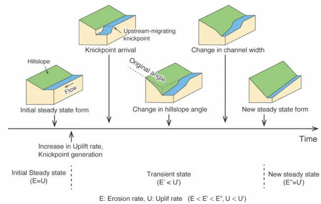
While it is steady-state river morphology that appropriately reflects the long-term uplift rates, it is also possible to extract tectonic information from rivers at a transient state by focusing on channels and hillslopes that have achieved their steady-state forms (e.g., Kirby and Whipple, 2012). A transient state refers to an intermediate state between one steady state to another (Fig. 1.2). The presence of an
upstream-propagating knickpoint is one diagnostic feature of a transient state (e.g., Wobus et al., 2006a). The occurrence of such knickpoint is widespread in tectonically-active regions, meaning it is necessary to understand transient river response to changes in tectonic activity and its timescales (e.g., Crosby and Whipple, 2006). Channel width and hillslope angle are major factors controlling erosion rates, and their morphological adjustment probably occurs after the passage of a knickpoint (e.g., Yanites, 2018) (Fig. 1.2). However, their response timescales were difficult to constrain because we cannot know when the response started and ended. There are only a few studies that estimated those timescales in actual landscapes. Therefore, I present a new approach to estimate timescales of width and hillslope adjustments based on the upstream migration speed of a knickpoint. Rates of knickpoint migration can be estimated theoretically (e.g., Whipple and Tucker, 1999; Royden and Perron, 2013). Field datasets have validated the predictive power of such theoretical rates (e.g., Crosby and Whipple, 2006; Berlin and Anderson, 2007). Results of my study suggest response timescales of width and hillslope can be several hundreds of thousands of years to ~1 My. Based on this result, I discuss how long it takes for a basin-scale steady state to be established and what we should do to infer more accurate uplift rates from river morphology.
5
Fig. 1.2. A schematic illustration of river response to an increase in uplift rates. A sustained increase in uplift rates (U to U’) generates a knickpoint that travels upstream through time. As the knickpoint migrates upstream, channel and hillslope downstream from the knickpoint starts to adjust their forms to the accelerated uplift rate, triggering a gradual increase in erosion rate (E to E’) (Transient state). This morphological adjustment continues until channel and hillslope achieve their steady-state forms, and the erosion rate balances with the uplift rates (New steady state).
Ch.2. Calibrating effects of rock strength on channel steepness to infer rock
uplift
2.1. Introduction
Current topography results from the interplay between rock uplift and erosion, meaning constraining uplift and erosion rates is important to understand landscape evolution. The concept of topographic steady state predicts erosion rate is adjusted to rock uplift rate (e.g., Hack, 1975; Willett and Brandon, 2002), and drives much attention to how erosion rate change depending on the imposed tectonics. Bedrock river plays a major role in modulating erosion rate by changing its morphology and setting the base level for hillslope that significantly affects sediment input to the river channel. The response of bedrock rivers to tectonics is controlled by various boundary conditions (e.g., tectonics, climate, substrate lithology), and disentangling their relationships is essential to estimate erosion rate from bedrock channel morphology and establish a reliable proxy of rock uplift rate. An advantage of using bedrock rivers is its ease of studying spatial uplift pattern, which is sometimes impossible for traditional approaches (e.g., identify offset markers and estimates uplift rates from their offset and ages) to achieve due to sparse distribution or poor preservation of offset markers.
Among various factors that influence erosion rate, channel slope is most often used to infer rock uplift rate from bedrock river morphology (e.g., Kirby and Whipple, 2012). The common detachment limited model predicts that erosion rate (&) is a function of channel slope (') and upstream drainage area ((: a proxy for flow discharge):
& = *(+'# (2.1)
where * is the erodibility coefficient, and 1 and 2 are positive constants (e.g., Howard and Kerby, 1983; Howard, 1994; Whipple and Tucker, 1999). The erodibility coefficient can vary by orders of magnitudes depending on hydrologic, climatic, and geologic boundary conditions, and has a large impact on river morphology and the response of river system to external forcing (e.g., Stock and Montgomery, 1999; Whipple and Tucker, 1999; Harel et al., 2016; Yanites et al., 2017). Therefore, when extracting tectonic information based on channel slope, contributions of other factors, such as substrate materials, channel width, and climate, to the erodibility coefficient must be considered (e.g., Duvall et al., 2004; Yanites, 2018; Adams et al., 2020).
7
such as tectonics, and there are various approaches to evaluate erosional resistance of rock (e.g., Selby, 1980; Sklar and Dietrich, 2001; Bursztyn et al., 2015; Goudie, 2016). Rock mass strength exerts primarily control over erosion rates, which was experimentally shown by Sklar and Dietrich (2001), who found that erosion rates inversely correlated with the square of rock tensile strength. In the field, rock mass strength is measured using a Schmidt hammer whose readings can be converted to uniaxial compressive strength (e.g., Selby, 1980; Bursztyn et al., 2015). Joints developed in a rock decreases the strength of rock depending on density, width, and orientations of joints, which influences the relationship between channel morphology and erosion rates (Molnar et al., 2007; DiBiase et al., 2018). The Selby rock mass strength (Selby, 1980) is a semi-quantitative measure of rock mass strength and considers intact rock strength, characteristics of joints, degree of weathering. Since various rock properties can affect erosion rates, a multivariate index like the Selby rock mass strength is useful to evaluate actual rock erodibility in the field (e.g., Whittaker et al., 2007; Goode and Wohl, 2010; Bursztyn et al., 2015). Although the indices mentioned above helps to examine whether observed differences in channel forms can be attributed to differential rock mass strength, it provides only qualitative evaluations rather than quantitative calibration within the stream power framework. This is because relationships between the indices of rock strength and the erodibility coefficient (* in Eq. 2.1) are probably highly dependent on local boundary conditions, and formulating such relationships would be extremely difficult. * can be directly calculated if erosion or uplift rates are already known (e.g., Snyder et al., 2000; Duvall et al., 2004; Gallen and Wegmann, 2017; Zondervan et al., 2020); however, such an approach is not possible when trying to estimate unknown uplift rates from channel forms.
In this study, we attempt to quantitatively calibrate dependency of channel slope on substrate lithology and reveal spatial uplift pattern along the Futagawa fault, a normal-dextral fault in southwestern Japan, using rivers flowing over various rock types. The steeper channel reaches correspond with outcrops of presumably resistant rocks in the study area, while gentler reaches are often associated with less resistant rocks. Our calibration method exploits work by Jansen et al. (2010), who stated that substrate erodibility could be inferred from the channel steepness index when rock uplift is spatially invariant. We estimated the ratio of substrate erodibility using basins that have experienced a similar uplift and calibrated effects of differential rock mass strength on channel slope (!"#: normalized channel steepness; Wobus et al., 2006). Based on calibrated !"#, we demonstrated that difference in rock erodibility, channel width, precipitation, and erosion process cannot explain the spatial distribution of !"# without differential
rock uplift.
2.2. Study area 2.2.1. Tectonic setting
Kyushu island is located in southwestern Japan, where the Philippine Sea plate subducts northeastward (N55°W) at 63–68 mm/yr relative to the overriding Amurian plate (Miyazaki and Heki, 2001) (Fig. 2.1). Decadal triangulation survey during 1891–1982 (Tada, 1984; 1985) and modern GPS network (Nishimura and Hashimoto, 2006) indicate central Kyushu is experiencing 1.3–1.4 mm/yr of north-south extension. In central Kyushu, lack of pre-Miocene basement and low Bouguer anomalies (Matsumoto, 1979; Kamata, 1985) indicates the NE-trending graben structure called the Beppu-Shimabara Graben (BSG, Matsumoto et al., 1979). The subducting Philippine sea plate mainly controls the tectonics and volcanic activity in the BSG (e.g., Kamata and Kodama, 1999; Mahony et al., 2011). According to Kamata and Kodama (1994, 1999), the Philippine sea plate resumed subduction at ~6 Ma after the halt or slowdown of subduction during 10–6 Ma, and the direction of subduction shifted from northwest to west-northwest at ~2 Ma (or 1.5–1 Ma: e.g., Nakamura et al., 1984). The resurgence of subduction at 6 Ma initiated N-S extension along the BSG and was followed by extensive volcanism in the central Kyushu (e.g., Kamata, 1985). Change in the direction of subduction at 2 Ma resulted in the transition of physical and chemical characteristics of volcanic activity and the formation of basins around central Kyushu (Itoh et al., 1998; Kamata and Kodama, 1999).
9
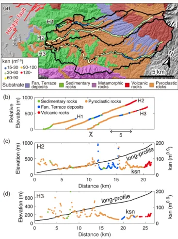
Figure 2.1. (a) Topography and (b) Geology of the study area. Inset map shows topography around Kyushu in southwestern Japan. Elevation data is from Geospatial Information Authority of Japan and National Centers for Environmental Information. Earthquake data is from the Japan Meteorological Agency earthquake catalog. Active fault traces are after Suzuki et al. (2017), Kumahara et al. (2017), and Nakata and Imaizumi (2002). Substrate lithology is from Hoshizumi et al. (2004, 2015). BSG: Beppu-Shimabara Graben. (c) Topography along X-X’. Takayubaru lava table is tilted toward the Futagawa fault by 1.5°.
The Futagawa fault is a northwest-dipping normal-dextral fault bounding the southern end of the BSG and accommodating north-south extension in central Kyushu (e.g., Matsumoto, 1979; Watanabe et al., 1979; Yano and Matsubara, 2017) (Fig., 2.1a). Surface traces of the Futagawa fault generally trends N53°E, which is oblique to the regional extensional axis (north-northwest to south-southeast: Matsumoto et al., 2018). Because of this obliquity, significant vertical displacement occurs along the Futagawa fault and is manifested by southeastward tilting of the lava plateau ejected from Omine at 116–87 ka (Takayubaru lave, Fig. 2.1b, 1c: Miyoshi et al., 2013). Ishimura (2019) estimated the right-lateral and vertical slip rate of the fault to be 1.5–3.7 mm/yr and 0.9–1.1 mm/yr, respectively. To the southeast of the Futagawa fault, there is another fault called the Idenokuchi fault, which is subparallel to the Futagawa fault (Fig. 2.1). The Idenokuchi fault is a normal fault dipping northwest by 50°–70° (e.g., Himematsu and Furuya, 2016; Toda et al., 2016), and its length is roughly half of that of the Futagawa fault. Both the Futagawa fault and the Idenokuchi fault ruptured in the Mw7.0 Kumamoto earthquake sequence in 2016 (e.g., Hashimoto et al., 2017) and were accompanied by surface ruptures with up to 2.2 m of dextral displacement and ~2 m of vertical displacement (e.g., Shirahama et al., 2016; Scott et al., 2018). The Mw7.0 event was preceded by the Mw6.2 event that produced minor surface ruptures around an intersection of the Futagawa fault and the Hinagu fault (e.g., Sugito et al., 2016). Hinagu fault is a right-lateral strike slip fault trending N25°E, and its dextral and vertical slip rate is 1.7–2.3 mm/yr at 10km to the south of Yamaide (Shirahama, 2020) and ~0.2 mm/yr at Yamaide (Okamura, et al., 2018), respectively.
2.2.2. Substrate rock types
Rivers around the epicentral area of the 2016 Kumamoto earthquake flow over contrasting substrates between the western and eastern part (Fig. 2.1b). In the western part, late Cretaceous sedimentary rocks, the Mifune group, are dominant, which are composed of massive clastic rocks (mainly sandstone and siltstone) and thin tuff beds (Kuroki et al., 1995; Saito et al., 2005; Ikegami et al., 2007). The Mifune group is more than 2,000 meters thick and unconformably overlies late Permian shale in the southernmost part of the study area (Hoshizumi et al., 2004; Tazawa et al., 2008). The Eastern part of the study area is characterized by late Quaternary volcanic rocks, welded tuff, and pyroclastic flow deposits. Rocks before ~0.3 Ma include andesitic lava units and tuff breccia, most of which are dated
11
volcanic rocks are covered by pyroclastic flow deposits and welded tuff related to four explosive eruptions that formed Aso caldera during 270–87 ka (e.g., Watanabe, 1972; Ono and Watanabe, 1983; Machida and Arai, 2003; Hoshizumi et al., 2004; Aoki, 2008). The Aso-4 eruption at 87 ka (Aoki, 2008) is the biggest event, and its pyroclastic flow traveled to 166 km away from the caldera; however, the deposits are now barely preserved within drainage basins we analyzed (Fig. 2.1b, Watanabe and Ono, 1969; Takarada and Hoshizumi, 2020). Pyroclastic rocks related to the Aso-2 (141±6 ka, Matsumoto et al., 1991) and the Aso-1 eruption (270-250 ka, Machida and Arai, 2003) outcrops in the basins of interest and consist of welded tuff and partially-welded scoria flow deposits (Hoshizumi et al., 2004). Metamorphic rocks occur around the basins F2, F3, and south of H3 (Fig. 2.1b, Hoshizumi et al., 2004). These include serpentinite (F2 and F3); Paleozoic schist (F3); and Mesozoic Schist (H3) (Hoshizumi et al., 2004; Osanai et al., 2014).
2.2.3. Basin characteristics
Rivers draining across the study area are mixed bedrock-alluvial rivers, characterized by frequent outcrops of bedrock at channel beds and walls but often covered by thin gravel layers (e.g., Howard, 1998). We focus on basins along the western part of the Futagawa fault (F1 to F3) and the Idenokuchi fault (F4 to F7) (Fig. 2.1, Table. 2.1). Areas between the Idenokuchi and the Futagawa fault are mostly filled with alluvium or engineered; Thus, we do not include in the analysis. Drainage areas of interest range between 2.1 and 74.5 km2 and their average is 8.3 km2.The study area has a temperate climate and receives an annual rainfall of ~2200 mm at lowland during 2003-2009 (Mashiki, 193 m a.s.l.) (Fig. 2.1a). From April to November of the same period, the mountainous area south of the Futagawa fault (Tawara-Yama, 850 m a.s.l.) (Fig. 2.1a) receives ~1.5-1.8 times more rainfall compared to the lowland (Japan Meteorological Agency, 2020). Precipitation data in a mountainous area south of the Futagawa fault (Tawara-Yama, 850 m a.s.l.) (Fig. 2.1a) covers only April to November during 2003-2009 but is ~1.5-1.8 times as large as that at lowland.
Table 2.1. Characteristics of basins and channel segments along the Futagawa and Hinagu fault. Basin/Segment ID Area (km 2) Critical area (km2) θ !"# Calibrated !"#a Calibrated !"#b F1 6.8 0.7 0.55 24 ± 6 24 ± 6 24 ± 6 F2 14.7 1.5 0.68 49 ± 12 50 ± 14 49 ± 13 F3 9.4 1.0 0.42 58 ± 15 51 ± 13 41 ± 17 F4 5.0 0.8 F4, 4-1 4.6 – 5.0 8.7 50 ± 10 47 ± 10 26 ± 5 F4, 4-2 2.9 – 4.1 -0.07 75 ± 13 65 ± 12 37 ± 6 F4, 4-3 0.8 – 2.5 0.46 22 ± 7 20 ± 7 11 ± 4 F5 15.2 1.1 F5, 5-1 4.3 – 15.2 0.76 118 ± 43 100 ± 37 58 ± 21 F5, 5-2 1.1 – 4.3 0.45 64 ± 9 60 ± 8 33 ± 5 F6 4.6 1.0 F6, 6-1 3.3 – 4.6 0.38 117 ± 22 93 ± 17 55 ± 10 F6, 6-2 1 – 3.3 0.53 78 ± 12 62 ± 10 37 ± 6 F7 2.1 1.0 -0.77 129 ± 39 102 ± 31 61 ± 18 H1 12.6 1.7 0.57 40 ± 13 H2 35.2 1.3 0.46 55 ± 12 H3 74.5 1.8 0.41 47 ± 14
!"#: mean and standard deviation. Those in bold and italics are shown in Fig. 2.3a. a Calculated using α (Table 2.3)
13 2.3. Methods
2.3.1. Longitudinal river profile and channel steepness
Longitudinal profile of a river channel at a steady state generally follows a power-law relationship between local channel slope (') and the drainage area upstream ((),
' = !"(34 (2.2)
where !" is the channel steepness index and 5 is the concavity index (e.g., Flint, 1974; Snyder et al., 2000). A similar relationship is derived from the detachment-limited model (Eq. 2.1). At a topographic steady state where local erosion rate balances with rock uplift rate (6) (e.g., Willett and Brandon, 2002), Eq. (2.1) is rewritten as ' = 76 *8 9 # (3+# (2.3)
From Eq. (2.2) and (2.3),
!"= 7 6 *8 9 # (2.4) 5 =1 2 (2.5)
Concavity index 5 typically falls between 0.4-0.6 at steady state and is generally independent of uplift rate (e.g., Kirby and Whipple, 2012). Calculating steepness index for basins using the same concavity index (5=>?) enables to infer regional uplift pattern (e.g., Snyder et al., 2000; Kirby et al., 2003; Wobus et al., 2006; Kirby and Whipple, 2012). In this case, channel steepness is referred to as normalized channel steepness (!"#).
We calculated !"# for rivers across the Futagawa and Idenokuchi fault (Fig 2.1, basins F1 to F7) to estimate long-term uplift trend along the faults. We used 10m DEM provided by Geospatial Information Authority in Japan. We defined the critical drainage area above which erosion process changes from colluvial to fluvial process using a local slope-area plot of each trunk stream (Stock and Dietrich, 2003). We extracted trunk streams using TopoToolbox 2 (Schwanghart and Scherler, 2014). To reduce noise inherent in the DEM, we subsampled points on the extracted channels at vertical intervals of 3 meters and calculated local slope and !"# using 5=>? = 0.45 (e.g., Wobus et al., 2006). We also calculated $ value and constructed $-elevation (@) plots (hereafter $-plot):
$ = A 7 (B ((C)8 + # D DE FC (2.6)
@(C) = @(CH) + J 6 *(B+K 9 # $ (2.7)
where C is horizontal upstream distance from an outlet, CH is the distance at the outlet (thus CH = 0 in this study), and (B is a reference drainage area and is set to be 1 in this study (Perron and Royden, 2013). Eq. (2.7) is the integral form of Eq. (2.2) assuming a steady state and spatially uniform 6 and *, and predicts that the slope of a $ plot represents a reach-averaged !"# when (B= 1, which helped us see if the extracted channels contain slope-break knickpoints (Whipple et al., 2013). Although the reach-averaged !"# is less noisy compared to local !"# calculated from Eq. (2.1) (Perron and Royden, 2013), we mostly used the latter to focus on the relation between local channel steepness and substrate rock types.
2.3.2. Calibrating rock erodibility
Effects of rock mass strength on channel steepness is one of the major complications when extracting tectonic information from channel morphology (e.g., Snyder et al., 2000; Kirby et al., 2003; Duvall et al., 2004; Allen et al., 2013; Bursztyn et al., 2015). Here we attempt to quantify the dependency of channel steepness on substrate lithology by calculating ratios of erodibility coefficient from normalized channel steepness of each substrates. As an example to explain the procedure, we use the basins F2 and F6, whose dominant substrate is sedimentary and volcanic rock, respectively (Fig. 2.1b). From Eq. (2.4), assuming the slope exponent 2 is independent of rock types as in previous studies (e.g, Duvall et al., 2004; Gallen and Wegmann, 2017; Yanites et al., 2017), !"# of the basin F2 and F6 is,
!"# OP = 76OP *Q>R8 9 # (2.8T) !"# OU= 76OU *VWX8 9 # (2.8Y) where subscripts 'ZF and [\] denotes sedimentary rocks and volcanic rocks, respectively. To compare uplift rates of basin F2 (6OP) and F6 (6OU) using !"#, Eq. (2.8b) has to be converted to
^39! "# OU= 7 6OU *Q>R8 9 # (2.9) *Q>R 9 # (2.10)
15
where ^ is a calibration factor. Eq. (2.8)–(2.10) predict that the difference in uplift rates between basins of different substrates can be estimated from the ratio of * for corresponding rock types. To derive the ratio of * for different substrates, we focus on basins H1-H3 draining across the Hinagu fault. Trunk streams of these basins merge downstream and intersect with the Hinagu fault at the same point, which suggests channel forms of these basins are adjusted to similar uplift rates (See Results for details). Assuming rock uplift rate 6 is uniform among basins H1 to H3, a ratio of the erodibility of different rock types (Eq. 2.10) can be written from Eq. (2.4) as the inverse ratio of !"# for corresponding rock types: ^ = 7*Q>R *VWX8 9 # = !"# VWX !"# Q>R (2.11)
Thus, we first calculated local !"# for basins H1 to H3 in the same way as for basins F1 to F7 and estimated calibration factors for each rock type. We calculated calibration factors so that ^ is one for sedimentary rocks, i.e. the denominator of Eq. 2.11 was always !"# for sedimentary rocks, while the numerator was !"# for any substrates other than sedimentary rocks. Therefore, ^ larger than one suggests the substrate is more resistant to erosion compared to sedimentary rocks, and ^ smaller than one means the substrate is less resistant. We used !"# averaged over reaches of each rock type in calculating ^. By using ^ of any combinations of rock types, we calibrated local !"# (Eq. 2.9) for basins F1 to F7.
2.3.3. Channel width measurement
Same as channel steepness, channel width varies depending on rock uplift rate and substrate erodibility (e.g., Montgomery and Gran, 2001; Duvall et al., 2004; Whittaker et al., 2007; Yanites and Tucker, 2010) and modulates the degree of adjustment of channel slope to imposed tectonics (e.g., Yanites, 2018). We measured channel width in selected basins to examine the contribution of channel width adjustment to observed !"# pattern. We measured high-flow width marked by vegetation boundaries, highest water-washed surface levels, and remains of flood debris (e.g., Whittaker et al., 2007; Zondervan et al., 2020). We chose reaches within basins F1, F2, and F6 where sedimentary rocks (F1 and F2) or volcanic rocks (F6) are dominant. The former rock type is presumed to be the weakest and the latter to be the strongest rock type among the three major rock types in the study area (Sedimentary, pyroclastic, and volcanic rocks) (e.g., Sklar and Dietrich, 2001). Thus, if reaches of these two rock types have similar channel
width, differences in !"# of those reaches can be attributed to channel slope adjustments rather than width. We also measured channel width using 0.5 m DEM that partially covers the study area. The DEM was created from 2 m DEM using bicubic spline interpolation. Because channel width depends on flow depth, which is impossible to be measured from DEM, DEM-based measurements were limited to reaches where the flow depth of nearby reach was measured in the field. We tested the accuracy of the DEM-based measurement by comparing it to the width measured in the field and confirmed that the errors were mostly within 20% of the actual width (Fig. 2.2).
2.4. Results
2.4.1. ksn along the Futagawa fault and the Idenokuchi fault
Normalized channel steepness is generally larger in the western part (!"#<60, F1 to F3) than in the eastern part (70<!"#, F4 to F7) (Fig. 2.3). Each river contains knickpoints with locally large !"#, and most of them do not correspond with kinks in $ plots (Fig. 2.4a). For example, in the basin F3, while knickpoints of various magnitude in size and degree occur frequently (Fig. 2.4b), its long-profile in the $ plot is almost linear (Fig. 2.4a), indicating the reach-average !"# is uniform over basin F3. On the other hand, basins F4 to F6 contain slope-break knickpoints at which a reach-averaged !"# changes markedly, which appears as kinks in the $ plot (Fig. 2.4a). The trunk stream of basin F4 consists of three segments of distinct steepness (Fig. 2.4a, 2.4c; Table 2.1).
17
Figure 2.2. Comparison of channel width measured in the field and using 0.5m DEM. Errors in DEM measurement are mostly less than 20%. The DEM is generated from 2 m DEM by bicubic spline interpolation. 5 10 15 20 25 Width, DEM (m) 5 10 15 20 25 Width, Field (m ) DEM : Field =1:11 : 0.8 0.8 : 1
Figure 2.3. Long-term uplift rates and vertical displacement of the Kumamoto earthquake along the Futagawa and the Idenokuchi fault. (a) Geology and !"# around the Futagawa and the Idenokuchi fault. Active fault traces are after Suzuki et al. (2017), Kumahara et al. (2017). Substrate lithology is from Hoshizumi et al. (2004, 2015). (b) Basin-average !"# and calibrated !"#. (c) Vertical slip rates along the Futagawa fault compiled from previous studies (See Table S2.1 for original data source). (d) Vertical displacement of the 2016 Kumamoto earthquake. Results of field measurements are from Okamura et al. (2018), and those of differential LiDAR are from Scott et al. (2018).
0 5 10 15 20 Distance (km) 0 100 ksn (m 0. 9) ksn Calibrated ksn 0 0.5 1 1.5
Vertical slip rate (mm/yr)
0 100 200 300 Vertical displacement (cm) 0 5 10 15 20 Distance (km) 0 100 ksn (m 0. 9) ksn Calibrated ksn 0 0.5 1 1.5
Vertical slip rate (mm/yr)
0 100 200 300 Vertical displacement (cm) 0 5 10 15 20 Distance (km) 0 100 ksn (m 0. 9) ksn Calibrated ksn 0 0.5 1 1.5
Vertical slip rate (mm/yr)
0 100 200 300
Vertical displacement (cm) Distance along N53°E (km)
Vertical slip rate
(mm/yr) Vertical displacement (cm) ksn (m 0.9 ) ksn (m0.9) (a) (b) (c) (d) Substrate 0 5 10 15 20 0 5 10 15 20 Fan, Terrace deposits Pyroclastic rocks Volcanic rocks Metamorphic rocks Sedimentary rocks 15-30 30-60 60-90 90-120 120-N N Active fault
Offset marker (Fig.3c)
F1 F1 F2 F2 F3F3 F4 F4 F5F5 F6 F6 F7 F7 F1 F2 F3 F4 F5 F6 F7
Field measurement LiDAR differencing Futagawa fault Futagawa fault Idenokuchi fault
19
Figure 2.4. Normalized channel steepness for trunk streams flowing across the Futagawa and the Idenokuchi fault. (a) $ plots. Dashed lines represent segment boundaries. (b)(c) Longitudinal profiles (black lines) and local !"# (colored points). (b-d) Color represents substrate lithology.
5 10 15 20 25 30 35 0 200 400 600 800 Relative Elevation (m) 0 2000 4000 6000 8000 10000 Distance (m) 0 200 400 600 Elevation (m) 0 50 100 150 ksn (m 0. 9) 0 1000 2000 3000 4000 5000 Distance (m) 200 300 400 500 600 Elevation (m) 0 100 200 300 ksn (m 0. 9) 5 10 15 20 25 30 35 0 200 400 600 800 Relative Elevation (m) 0 2000 4000 6000 8000 10000 Distance (m) 0 200 400 600 Elevation (m) 0 50 100 150 ksn (m 0. 9) 0 1000 2000 3000 4000 5000 Distance (m) 200 300 400 500 600 Elevation (m) 0 100 200 300 ksn (m 0. 9) F3 F1 “F4, 4-1” Segment boundary Basin/Segment ID (Table 1) 4-1 4-2 4-3 5-1 5-2 6-2 6-1 F2 F3 F4 F5 F6 F7 ksn long-profile Substrate Sedimentary rocks Terrace deposits Volcanic rocks Metamorohic rocks Pyroclastic rocks F4 5 χ ksn Fault long-profile (b) (a) (c)
Given the relationship between rock mass strength and erosion rate (e.g., Sklar and Dietrich, 2001), intra- and inter-basin lithologic contrasts should contribute to the observed !"# pattern around the Futagawa fault. According to the abrasion mill experiment (Sklar and Dietrich, 2001), clastic sedimentary rocks that typically occur in the western part (F1 to F3) are generally more erodible than andesite and welded tuff dominant in the eastern part (F4 to F7). Mafic schist, which occurs in basin F3, is more resistant to erosion than clastic sedimentary rocks (Sklar and Dietrich, 2001). Contrasts in substrate rock erodibility can cause differential channel steepness or generate a knickpoint at a lithologic boundary. However, based on our visual inspection, neither of these were identified in basins F1 to F7. For example, at around 5000 meters from the outlet of the basin F3, the substrate changes from sedimentary rocks to green schist (Fig. 2.4b). Although local !"# for the reaches underlain by green schist fluctuates widely due to frequent knickpoints, its reach-average !"# determined from the $ plot (59.0–61.2, 95% confidence interval) is quite similar to that of the sedimentary rock reaches (54.4–57.3). Likewise, in the further upstream of basin F3, reach-average !"# of the andesitic reaches is 48.3–51.8 and is slightly smaller than that for reaches of sedimentary rocks downstream, which does not agree with an expectation that the harder andesite should be associated with higher steepness than sedimentary rock. This is partly because the upstream part of basin F3 is still in transient state as is suggested by the smaller !"# values (~30) in the uppermost reach. Nevertheless, the !"# in basin F3 does not change as expected from the difference in intact rock mass strength between sedimentary rocks and andesite (Sklar and Dietrich, 2001), suggesting intact rock mass strength is not the only control on channel steepness (e.g., Whipple and Tucker, 1999, 2002).
2.4.2. ksn dependency on substrate rock types
To estimate dependency of !"# on substrate rock type, we calculated !"# for basins along the Hinagu fault: H1 to H3. The resulting !"# range mostly between 30 and 80 and up to ~860 (Fig. 2.5, S2.1). Average !"# of H1 to H3 are slightly different, but overlap within 1σ range (Table 2.1). These rivers contain many knickpoints (or zones), but those knickpoints did not always occur at lithologic boundaries nor within reaches of a specific rock type. Some of the observed knickpoints occur as waterfalls and are vertical-step knickpoints, while some others form boundaries at which reach-average !"# changes: thus slope-break knickpoints (e.g., Whipple et al., 2013).
21
Figure 2.5. Normalized channel steepness for trunk streams flowing across the Hinagu fault. (a) Substrate geology and !"#. Active fault traces are after Kumahara et al. (2017). (b) $ plots. (c)(d) Longitudinal profiles (black lines) and local !"# (colored points). (b-d) Color represents substrate lithology.
For example, downstream reaches of basin H2 (distance < ~5 km in Fig. 2.5c) exhibits larger !"# values compared to its upper reaches. If this change in !"# is related to tectonic activity, similar change in !"# should be observed for basin H1 and H3 because basins H1 to H3 cross the Hinagu fault almost at the same point (Fig. 2.5a). However, both H1 and H3 do not contain such slope-break knickpoints (Fig. 2.5b, S2.1). Also, the uppermost part of basin H2 has comparable !"# to the reach near the outlet, suggesting relatively larger !"# near the outlet of basin H2 is related to local geologic condition rather than tectonic activity.
Figure 2.6 illustrates the relation between !"# and distance from the Futagawa or Hinagu fault to points on the trunk streams where !"# are calculated. If basins H1–H3 have been subjected to spatially non-uniform uplift caused by the faults, !"# would decrease with the increase in the distance from the faults. However, there is no such correlation, which suggests the basins H1 to H3 have been experiencing spatially uniform uplift.
We calculated the average !"# for each rock type that occurs within basin H1-H3 to estimate !"# typical to each rock type. Because trunk rivers of basin H1-H3 contain knickpoints whose channel steepness (100–860) is much greater than typical values (30–80), averaging !"# over entire reaches fails to capture representative steepness of each rock type (Table 2.2). To eliminate reaches of anomalously high steepness, we restrict our analysis to !"# < 80, which excludes 16% of the dataset. The threshold steepness was determined to eliminate as many knickpoints as possible from the dataset while retaining ordinary reaches that have steepness typical of each substrate. As is
expected from the difference in rock tensile strength (Sklar and Dietrich, 2001), reaches of
sedimentary rocks are gentler than those of pyroclastic rocks and volcanic rocks (Fig. 2.7, Table 2.2). Reaches of pyroclastic rocks are slightly steeper than those of sedimentary rocks, probably because they include both relatively weak scoria flow deposits and welded tuff that is as resistant as andesite to erosion (Sklar and Dietrich, 2001). Reaches of terrace deposits occur in a very limited area (n=9, Fig. 2.7) and are the gentlest among four substrates examined.
23
Figure 2.6. Relation between !"# for basins H1–H3 and distance from (a) the Futagawa and (b) the Hinagu fault.
2 4 6 8 10 12 14
Distance from the Futagawa fault (km) 0 50 100 150 200 k sn H1 H2 H3 5 10 15 20
Distance from the Hinagu fault (km) 0 50 100 150 200 k sn H1 H2 H3 (a) (b)
Table 2.2. !"# for dominant substrates within basins H1 to H3 Geologic unit Count a !
"# a Count b !"# b
Terrace deposit 9 32 ± 8 9 32 ± 8
Sedimentary rock 64 121 ± 166 37 46 ± 13
Volcanic rock 59 58 ± 13 57 58 ± 12
Pyroclastic rock 296 66 ± 82 256 49 ± 14
!"#: mean and standard deviation. a All data
b Calculated from !
25
Figure 2.7. Histograms of !"# for each rock type calculated from basins H1–H3. Bin width is 2.
Terr, n=8 0 50 100 ksn (m0.9) 0 0.1 0.2 Probability Fan, n=42 0 50 100 ksn (m0.9) 0 0.1 0.2 Probability Sedi, n=30 0 50 100 ksn (m0.9) 0 0.1 0.2 Probability Volc, n=48 0 50 100 ksn (m0.9) 0 0.1 0.2 Probability WTuff&Pmc, n=214 0 50 100 ksn (m0.9) 0 0.1 0.2 Probability Allu, n=10 0 50 100 150 200 250 ksn (m0.9) 0 1 2 Count Fan, n=53 0 50 100 150 200 250 ksn (m0.9) 0 5 Count Sedi, n=34 0 50 100 150 200 250 ksn (m0.9) 0 5 Count Volc, n=60 0 50 100 150 200 250 ksn (m0.9) 0 5 Count WTuff&Pmc, n=262 0 50 100 150 200 250 ksn (m0.9) 0 10 20 Count Allu, n=10 0 50 100 150 200 250 ksn (m0.9) 0 1 2 Count Fan, n=53 0 50 100 150 200 250 ksn (m0.9) 0 5 Count Sedi, n=34 0 50 100 150 200 250 ksn (m0.9) 0 5 Count Volc, n=60 0 50 100 150 200 250 ksn (m0.9) 0 5 Count WTuff&Pmc, n=262 0 50 100 150 200 250 ksn (m0.9) 0 10 20 Count Allu, n=10 0 50 100 150 200 250 ksn (m0.9) 0 1 2 Count Fan, n=53 0 50 100 150 200 250 ksn (m0.9) 0 5 Count Sedi, n=34 0 50 100 150 200 250 ksn (m0.9) 0 5 Count Volc, n=60 0 50 100 150 200 250 ksn (m0.9) 0 5 Count WTuff&Pmc, n=262 0 50 100 150 200 250 ksn (m0.9) 0 10 20 Count Allu, n=10 0 50 100 150 200 250 ksn (m0.9) 0 1 2 Count Fan, n=53 0 50 100 150 200 250 ksn (m0.9) 0 5 Count Sedi, n=34 0 50 100 150 200 250 ksn (m0.9) 0 5 Count Volc, n=60 0 50 100 150 200 250 ksn (m0.9) 0 5 Count WTuff&Pmc, n=262 0 50 100 150 200 250 ksn (m0.9) 0 10 20 Count Allu, n=10 0 50 100 150 200 250 ksn (m0.9) 0 1 2 Count Fan, n=53 0 50 100 150 200 250 ksn (m0.9) 0 5 Count Sedi, n=34 0 50 100 150 200 250 ksn (m0.9) 0 5 Count Volc, n=60 0 50 100 150 200 250 ksn (m0.9) 0 5 Count WTuff&Pmc, n=262 0 50 100 150 200 250 ksn (m0.9) 0 10 20 Count Count Terrace deposits Sedimentary rocks Volcaninc rocks Pyroclastic rocks
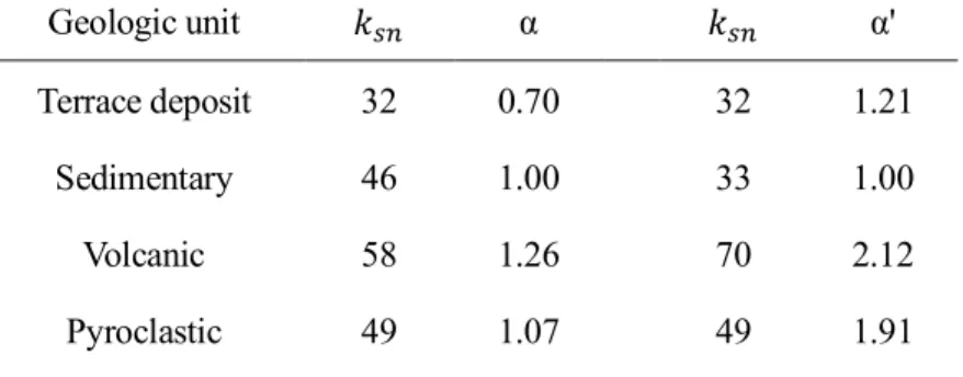
Using resulting !"# values, we calculated calibration factors (Eq. 2.11). Table 2.3 shows two sets of calibration factors (^ and α'). Those on the left (α) were calculated from average !"# for each rock type and used to calculate calibrated !"# plotted on Fig. 2.3. Those on the right (α') were based on the assumption that sedimentary rocks were much weaker than the other rocks, and were calculated using the minimum !"# within 1σ range for sedimentary rocks and the maximum !"# within 1σ range for volcanic and pyroclastic rocks. Because metamorphic rocks do not crop out along trunk streams of basins H1–H3 and we cannot calculate α, we used α of volcanic rocks for mafic schists and that of sedimentary rocks for serpentinite based on rock tensile strength (Mambetov and Mosinets, 1965; Sklar and Dietrich, 2001). We used calibration factors α' (Table 2.3) to see whether the observed !"# pattern along the Futagawa and the Idenokuchi fault could be explained solely by differential erodibility of substrate materials.
Calibrated !"# in the eastern part (F4–F7) decreased by 10–30 compared to pre-calibration steepness, and were still larger than in the western part (F1–F3) (Fig. 2.3a). Even when assuming sedimentary rocks are much weaker than volcanic and pyroclastic rocks (thus, when using α' in Table 2.3), !"# in the eastern part was as large as or slightly larger than in the western part, which indicates that observed difference in !"# between the east and west cannot be explained only by lithologic contrasts.
2.4.3. Channel width dependency on lithology
Channel width of reaches underlain by sedimentary rocks (basins F1 and F2) follows a typical hydraulic scaling where channel width increases with drainage area raised to the power of 0.3-0.5 (e.g., Montgomery and Gran, 2001; Whipple, 2004) (Fig. 2.8). Reaches of volcanic rocks (basin F6) have similar width to those of sedimentary rocks, although it is uncertain whether the data can be regressed to the typical scaling due to the small sample size (n=8).
2.5. Discussion
We demonstrated that the observed !"# pattern in the study area could not be attributed solely to differences in the erodibility of substrate materials. Here we first discuss other factors that potentially contribute to the observed !"# (channel width, climate, erosion process), and move to tectonic implications.
27
Table 2.3. Calibration factor and corresponding !"# for dominant substrates Geologic unit !"# α !"# α'
Terrace deposit 32 0.70 32 1.21
Sedimentary 46 1.00 33 1.00
Volcanic 58 1.26 70 2.12
Figure 2.8. Channel width for reaches of sedimentary rocks and volcanic rocks. 106 107 Drainage area (m2) 5 10 15 20 25 30 Width (m) Sedimentary rocks (n=42) Volcanic rocks (n=8) 106 107 Drainage area (m2) 5 10 15 20 25 30 Width (m) Sedimentary rocks (n=42) Volcanic rocks (n=8) 106 107 Drainage area (m2) 5 10 15 20 25 30 Width (m) Sedimentary rocks (n=42) Volcanic rocks (n=8) Drainage area (m2) W = 5.5A0.49
29 2.5.1. Channel width
Channel width measured in the field and from DEM shows that reaches of sedimentary rocks and volcanic rocks have similar width (Fig. 2.8), which implies that the observed difference in !"# between reaches of sedimentary and volcanic rocks does not result from the difference in channel width. A potential complication concerning this implication is that reaches of volcanic rocks (basin F6) are at a transient state as suggested by the presence of a slop-break knickpoint (Fig. 2.4a, Table 2.1), suggesting channel width measured in basin F6 might not be adjusted to the current tectonic condition yet. According to a numerical model that assumes “sediment cover detachment-limited” condition where river bed is partially covered by alluvium (Yanites, 2018), channel width becomes narrower soon after a passage of a knickpoint. As the knickpoint propagates upstream, local sediment supply increases and greater portion of the bed will be covered by sediments, causing long-lived widening (e.g., Yanites, 2018; Yanites and Tucker, 2010). Based on the modeling results, channel width observed in basin F6 will probably become wider, which means even steeper channel gradient will be required for the local erosion rate to catch up with the uplift rate (e.g., Eq. 2.14 in Yanites, 2018). Therefore, even if channel width for volcanic rocks reaches becomes wider than that of sedimentary rock reaches in the future, that will increase !"# of volcanic rock reaches and not affect our interpretation that differential rock uplift in the study area is mainly responsible for the observed !"# distribution.
2.5.2. Precipitation
Based on precipitation data at lowland (Mashiki, Fig. 2.1a) and a mountainous area (Tawara-Yama, Fig. 2.1a), basins closer to Aso caldera receive more rainfall than those farther from the caldera. Increasing rainfall (discharge) at a given point on a river will enhance the erodibility, resulting in a decrease in channel gradient required for local erosion rate to match rock uplift rate (e.g., Roe et al., 2003; Bookhagen et al., 2012; Adams et al., 2020). Therefore, if we could calibrate !"# in terms of the effect of precipitation, average !"# in the eastern part of the study area would increase relative to those in the western part, which further enlarge the difference in !"# between the east and west of the study area.
2.5.3. Erosion process
standard detachment-limited model (Eq. 2.2) was independent of substrate rock type as was commonly assumed (e.g, Duvall et al., 2004; Gallen and Wegmann, 2017; Yanites et al., 2017). This assumption may not hold true in our study area where substrate rock is not uniform because 2 reflects the dominant erosion process controlled by substrate properties (e.g., Hancock et al., 1998; Wohl, 1998; Whipple et al., 2000). An exponent 2 governs the relationship between erosion rate and basal shear stress and has profound effects on river response to imposed tectonic force (e.g., Whipple and Tucker, 1999; Tucker and Whipple, 2002; Mitchell and Yanites, 2019). Although our field observation confirmed that both abrasion and plucking occurred in reaches of sedimentary and volcanic rocks (Fig. 2.9), reaches of sedimentary rocks tended to exhibit polished and smooth surfaces while those of volcanic rocks often had rugged and plucked surfaces.
If we assume the erosion process operative on sedimentary rocks and volcanic rocks is abrasion and plucking, respectively, a ratio of erodibility coefficients can be written from Eq. (2.4):
*VWX *Q>R=
!"# Q>R#abc
!"# VWX#def (2.12)
where 2Q>R and 2VWX are 5/3 and 2/3–1, respectively (Whipple et al., 2000). Also, a ratio of uplift (erosion) rate between basin F2 where sedimentary rocks are dominant and F6 where volcanic rocks are dominant can be written using Eq. (2.8):
6OU 6OP =
*VWX!"# OU#def
*Q>R!"# OP#abc (2.13)
From Eq. (2.12) and average !"# for basin F2 and F6, the uplift ratio (Eq. 2.13) can be calculated as 0.73–1.82 (Table 2.4). Therefore, even if the erosion process is totally different between reaches of sedimentary and volcanic rocks, relative uplift rates in the eastern part are greater than or almost same as those in the western part.
31
Figure 2.9. Photographs of mixed bedrock-alluvial rivers in the study area. (a) Abraded surface of siltstone. (b) An outcrop of blocky siltstone where plucking occurs probably along bedding planes. (c) Relatively smooth andesite is exposed at channel wall. The channel bed is mostly covered with gravel at this point. (d) Highly jointed andesite exposed at channel bed. Bedform is generally rugged, but less-jointed areas tend to exhibit smooth surfaces.
Table 2.4. Uplift rate ratio between F2 and F6 !"# VWX !"# Q>R 2VWX 2Q>R 6OU/6OPa 58 46 0.67 1.67 1.44 58 46 1.00 1.67 1.82 70 33 0.67 1.67 0.73 70 33 1.00 1.67 0.86 a From Eq. (2.13).
33
2.5.4. Implications for long-term relative uplift and earthquake recurrence
We showed that the spatial distribution of !"# was difficult to explain without differential long-term uplift rates in the study area. However, current stream analysis cannot capture relative uplift along the eastern part of the Futagawa fault because bedrock is not exposed at the footwall-side of the fault. To reveal the along-strike variation of vertical slip rates of the Futagawa fault, we compiled slip rates from published papers and reports (Fig. 2.3c; Table S2.1). Offset markers were lava units and pyroclastic flow deposits dated between 270–90 ka (Table S2.1). Given the earthquake recurrence interval of the Futagawa fault is approximately two or three thousand years (Ishimura et al., 2020), the offset markers are old enough to derive average slip rate of the fault (Styron, 2019). Vertical slip rates showed the same trend as channel steepness: 0.7–1.0 mm/yr in the east and 0.4–0.5 mm/yr in the west (Fig. 2.3c). This result, together with the spatial distribution of channel steepness, indicates relative uplift rates in the eastern part of the study area probably outpace those in the western part in the last 270–90 ky.
The long-term differential uplift between the east and the west may reflect crustal deformation related to the volcanic activity of Mt. Aso, which is located at ~10 km to the northeast from basin F1 (Fig. 2.1) and one of the largest active volcanoes in Japan. If that is the case, channel steepness is expected to increase toward the caldera. However, there is no such increase occurring within basins H1–H3 (Fig. 2.5b; Fig. S2.1), which suggests that volcanic deformation does not have discernible effects on the observed channel steepness. Therefore, long-term relative uplift inferred from !"# results primarily from tectonic deformation occurring along the Futagawa and the Idenokuchi fault.
The distribution of long-term relative uplift rates is comparable to vertical displacements during the 2016 Kumamoto earthquake along the Futagawa and the Idenokuchi fault. Along the Futagawa fault, vertical displacements measured in the field (Shirahama et al., 2016; Okamura et al., 2018) were mostly less than 50 cm. Remote sensing analysis (pre- and post-earthquake lidar-differencing, Scott et al., 2018; SAR pixel offset, Himematsu and Furuya, 2020) revealed that maximum vertical displacement was ~200 cm, with its peak occurring at ~13–14 km in Fig. 2.3d. Vertical displacements along the Idenokuchi fault increased to the northeast and reached as large as 290 cm in the field measurement (Okamura et al., 2018), which is much larger than that estimated from SAR pixel offset (~100 cm, Himematsu and Furuya, 2020). This discrepancy in the vertical displacement is probably because it occurred on a steep hillslope and within a fault bend, both of which tend to exaggerate vertical displacement (e.g., Huang et al., 2017; Iezzi et al., 2018). To sum up, in the 2016 earthquake, vertical displacement in the eastern part of the
study area was much larger than that in the western part.
The similarity between the long-term uplift and the distribution of vertical displacement of the 2016 event has important insight into the earthquake recurrence of the Futagawa fault. Neither fault creep nor significant post-seismic displacement compared to co-seismic displacement was observed along the Futagawa and the Idenokuchi fault (Himematsu and Furuya, 2020), which suggests the long-term uplift rates represent sum of co-seismic displacement of individual earthquakes. Therefore, based on the similarity between the long-term uplift rates and the 2016 vertical displacement, we infer vertical slip distribution of the 2016 event is typical of earthquakes caused by the Futagawa fault.
2.5.5. Limitation of our approach
Our current method assumes that the erodibility coefficient * solely depends on strength of substrate rock. This means the current approach fails to calibrate * when channel slope is primarily controlled by the ability of a river transporting the sediment load rather than that detaching particles from the bed rock (e.g., Howard, 1998; Sklar and Dietrich, 1998). Effects of sediment load on erosion rate are often considered using a ratio of bedload sediment flux to transport capacity (e.g., Sklar and Dietrich, 1998; Whipple and Tucker, 2002; Yanites, 2018). As the ratio increases from 0 to 1, the river approaches from detachment limited to transport limited condition where steady-state channel slope becomes insensitive to properties of substrates (e.g., Sklar and Dietrich, 2006; Johnson et al., 2009). These two end-member conditions have marked differences in how a channel responds to changes in boundary conditions (e.g., relative uplift rate, substrate lithology). The detachment limited model predicts that tectonic signals or contrasts in substrate erodibility appear as a prominent knickpoint in a long-profile, while the transport limited model predicts that more gradual adjustment of channel gradient (e.g., Whipple and Tucker, 2002; Yanites, 2018). In our study area, frequent occurrence of abrupt knickpoints and the difference in channel steepness depending on rock types indicates that the rivers are probably inclined to detachment-limited condition. Although quantifying or calibrating the effect of sediment load based on actual field data is still difficult (e.g., Cowie, et al., 2008), striking differences in transient long-profiles helps to distinguish whether rivers of interests are favored by detachment- or transport-limited condition (e.g., Whipple and Tucker, 2002).
35 2.6. Conclusions
We revealed spatial distribution of long-term relative uplift rates along the Futagawa and the Idenokuchi fault based on calibrated !"# that considered the effects of substrate erodibility on channel steepness. Relative uplift rates inferred from calibrated !"# as well as vertical slip rates along the Futagawa fault suggests that there is a clear difference in uplift rates between the eastern and the western part of the study area. This long-term trend corresponds with the vertical displacement during the 2016 Kumamoto earthquake, suggesting that earthquakes of similar vertical slip distribution to the 2016 event repeatedly occurred along the Futagawa fault.
Our quantitative calibration method is useful under a detachment-limited condition where an erosion rate is primarily controlled by substrate erodibility. When substrate properties other than intact rock mass strength (e.g., joints, weathering) have profound influences on channel slopes, calibration factors estimated from local !"# probably reflects such effects. One potential limitation of our approach is that accuracy of calibration will decrease as sediment supply increases and the river system approaches a transport-limited condition. Thus, although our approach enables quantitative evaluation of the effects of substrate erodibility on channel morphology, careful inspection of longitudinal channel profiles and its relation to substrates is indispensable.
Ch. 3. Response timescales of channel width and hillslope angles to
accelerated incision estimated from a knickpoint travel time
3.1. Introduction
River erosion into bedrock controls the shape of mountainous landscapes, and quantifying erosion rates and its response to external forces such as climate and tectonics is fundamental to understand landscape evolution. Morphologies of channels and hillslopes at a topographic steady state (e.g., Willett and Brandon, 2002) dictate erosion rates, and establishing their functional relationships received much attention from geomorphologists (e.g., Ahnert, 1970; Whipple and Tucker, 1999; Roering et al., 2007). A topographic steady state is achieved when an erosion rate is in equilibrium with a rock uplift rate, meaning steady-state river morphologies can be a proxy for rock uplift rates (e.g., Wobus et al., 2006a; Kirby and Whipple, 2012). A sudden increase in uplift rates can increase local erosion rates, and channel and hillslope gradually respond to the accelerated erosion as the tectonic signal propagates upstream as a knickpoint (e.g., Whipple and Tucker, 1999; Crosby and Whipple, 2006). The presence of knickpoints is very common for rivers draining across tectonically active areas, and thus knowledge of transient response of rivers to tectonics and their response timescales is important to extract tectonic information from river morphologies.
Channel slope, width, and hillslope angle are major factors controlling erosion rates, and their response to changes in tectonic forces was studied both theoretically and empirically (e.g., Whipple and Tucker, 1999; Snyder et al., 2000; Yanites and Tucker, 2010; Lavé and Avouac, 2001; Roering et al., 2001; Reinhardt et al., 2007; Montgomery and Brandon, 2002). For example, channel steepness, a proxy for channel slope (e.g., Snyder et al., 2000), increases in the wake of a propagating knickpoint. Channel steepness downstream from the knickpoint is assumed to reach a new steady state and is proved to have a positive correlation with uplift rates (e.g., Kirby and Whipple, 2012; Regalla et al., 2013; Chen et al., 2015; Gallen and Wegmann, 2017). The response of channel width and hillslope seems to be more complicated than that of channel slope. Channel can become wider or narrower in response to tectonics or independent of uplift rates (e.g., Lavé and Avouac, 2001; Snyder et al., 2003; Yanites and Tucker, 2010). According to numerical modeling that considers the effects of sediment cover (Yanites, 2018), a channel first narrows after the passage of a knickpoint. It gradually widens as the knickpoint travels