An Heuristic Approach to Acceptance Rules in Integrated Scheduling Systems

(1)

J. Operations Research Soc. of Japan Vo!. 16, No. 1, March 1973

AN HEURISTIC APPROACH TO ACCEPTANCE RULES

IN INTEGRATED SCHEDULING SYSTEMS

KEINOSUKE ONO Keio University

CURTIS H. JONES The Peace Corporation (Received April 7, 1972)

Abstract

The development of integrated manufacturing systems demands a more complete understanding of the order acceptance and promise date establishment processes. This article uses a job shop simulation to explore the effects of various heuristic acceptance rules on a

manu-facturing facility. The Effective Gradient Method of Senju and

Toyoda, and a modification of that technique to include consideration of delivery commitments are combined with a variety of sequence decision rules and overtime decision rules to permit an examination of the interactions between the rules.

The results show the beneficial effects of including delivery, capacity, and profit considerations in the acceptance process. A study of the effects of different assumptions on the effective operating rate shows that all of the heuristic rules are over-simplifications of the complex relationships between particular decisions and the profit of the shop. The article suggests the formation of more complex rules and the development of operating systems which allow a decision maker to simulate a number of alternative combinations of rules to find one which fits his situation.

36

(2)

Despite early assertions by such experts as Conwayand Maxwell [1] that" decisions in planning and loading are of greater consequence," the mass of the extensive academic research effort on the job shop is still concentrated on the sequencing or dispatching function, "which job should be scheduled on this machine next." There have been very few attempts to develop decision rules on short·term capacity adjustments or on the selection of jobs to be accepted.

Senju and Toyoda [9] are the first authors we are aware of to deal with the problems of order acceptance. Their work suggests some obvious parallels between order acceptance decisions and se-quencing decisions. In both cases academic research began with the demonstration that the problem could be defined as an integer

pro-gramming problem. In the case of order acceptance, as in the

sequencing problem, the size of the tableau raises computational requirements beyond the capabilities of the computer resources which .can be presumed to be available to solve real industrial problems. Just as Rowe [8], Jackson [6], Conway, Maxwell, and Miller [2], and Gere [4], and others have gone on to propose useful heuristics, Senju and Toyoda have developed an effective gradient method which is designed to effectively represent the various capacity constraint equations of an integer program.

Acceptance Rules as Part of an Integrated System

An understanding of acceptance decisions and their relations with ,other production planning decisions is becoming increasingly important due to the tremendous effort and interest in the development of integrated manufacturing information systems. The large computer firms have put hundreds of man-years into PICS (IBM), GEMMAC (GE), and other such systems. Scholars such as Hosltein [5] have tried to build cohesive conceptual schemes around the integrated set of decisions involved in such a system,

(3)

38 Kein08uke Ono and Gurti8 H. Jone8

Most of these systems provide simple connections between certain islands of sophisticated treatment. They tend to provide considerable detail for such well-studied tasks as dispatching rules, inventory models, forecasting, and precedence diagrams. Few, if any, of them pay detailed attention to the task of which orders with their ac-companying contributions, promise dates, and penalty structures, should be accepted in the light of existing and expected shop loads and capacities.

In an effort to help systems designers to more effectively integrate the order acceptance process into the total production planning system, this article will explore the effect of different acceptance rules on the total system. In particular, it will examine Senju and Toyoda's effective gradient method of order acceptance and a modification of that method in a simple scheduling environment. It is the authors' hope that an examination of these results will encourage systems designers to consider alternative rules of order acceptance and to make more accurate predictions about their probable effects.

The authors wished to explore the effects of different acceptance policies in combination with different dispatching and overtime policies in the context of a simulated small deterministic job shop.

The Environment

The "What would happen if" look ahead feature of the job shop scheduling model developed by Ferguson and lones [3], and modified by lones, Hughes, and Engvold [7] provides a suitable framework for performing our examination of the effects of different acceptance rules. Although the model was devised to facilitate human inputs to a man-computer system, the ability to tryout different acceptance rules, different short-term capacity rules, and different sequencing rules, are useful in an automatic series of trials with no human modifications. The interrelationships of the rules can be brought out

(4)

1 Job 1

Opera~ion

# 1 No_ I Mach_I Hours

opera~ion

# 21

opera~ion

# 31

opera~ion

# 4 \ Operation # 51

M~~:;al

11 H 7 B(3) 10 L 5 B(l) 5 500 610 1 12 H 9 B(3) 8 L 9 B(2) 2 L 1 450 790 5 13 H 9 B(l) 4 G 4 B(3) 8 G 5 140 880 1 14 L 8 G 6 B(2) 6 G 5 120 910 4 15 B(l) 7 H 3 B(2) 6 G 9 H 7 210 800 3 16 G 3 H 7 L 5 H 4 200 670 3 17 L 1 H 7 L 8 B(l) 5 180 670 2 18 H 1 B(l) 10 G 5 H 5 G 7 360 870 4 19 L 3 H 6 B(3) 3 H 3 L 9 150 710 2 20 H 7 B(3) 9 H 3 B(3) 3 G 10 250 840 4 ~ ;:s ~ !::

...

;.

...

;;. ~

:g

2 ...

:r

...

Q ~

g

~ Q ;:s

...

~ ~ !::

-~

...

(5)

40 Keinosuke Ono and Curtis H. Jones

by trying different combinations.

The following list of essential characteristics of the shop will help to understand the environment in which the various acceptance rules were evaluated. A more complete description is available in Jones, Hughes, and Engvold.

A. The production system consists of six machines: a lathe, a grinding machine, two boring machines, and two heat treating furnaces.

B. Ten or twenty jobs are available for acceptance at the beginning

of the schedule period. Each job has associated with it a sales price, a raw material cost, a promise date, and three to five specified ope-rations. Table 1 shows these data for order sets

*I

1 and

*I

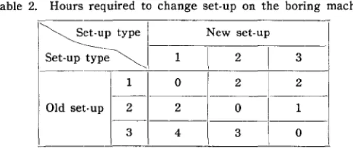
2.

C. The boring machines require variable set-up times, depending on the requirement of successive jobs. The time to change setups is shown in Table 2.

Table 2. Hours required to change set-up on the boring machine.

~et-up type New set-up

Set-up

;;~

1

_I

2

_I

3

1 0 2 2

Old set-up 2 2 0 1

3 4 3 0

D. Overtime costs vary by machine type. The lathe, grinder, boring machine and heat treat furnace cost seven, five, twelve, and fifteen dollars per hour respectively. Overtime costs are charged from the end of the regular shift until the completion of the overtime work. Overtime may not exceed eight hours per day.

(6)

for operations completed unless the job is finished. For each day that the job is late, a $ 200 penalty is subtracted from the price. The cost of operating the machines in the regular shift is considered fixed ($ 320 per day). For each job accepted, a sales expense item of $ 50 is charged.

F. The task is to maxmize profits over a three-day planning horizon. As stated before, this experiment is concerned with the three major aspects of operation management activity: (1) selection of the jobs to be accepted from the set available, (2) production capacity adjust-ment through the assignadjust-ment of overtime hours, and (3) sequencing, or dispatching, jobs to machines.

The computer program, as we used it, is a simulation routine. Three kinds of rules are required to carry out the simulation. In order to process (i.e., accept or reject) a new order, the computer must be instructed as to the criteria or rule to be applied. Similarly, a rule must be provided to allow the computer to determine how much overtime must be worked on each machine each day. Finally, when there is an idle machine and more than one job is ready to be per-formed on that machine, the compute!" must have a rule to determine which job to schedule first.

The computer program includes a choice of acceptance rules {ARULE's), overtime hour rules (HRULE's), and scheduling rules (SRULE's). The operator selects the rules by assigning values to HRULE, ARULE, and SRULE.

Acceptance Rule

Our program included two of Jones, Hughes, and Engvold's ARULES. ARULE=l called for the acceptance of all orders. ARULE =2 provided a check on the profitability of the orders by checking to see that the order would still show a profit if completed on over-time.

(7)

42 Keinosuke Ono and Curtis H. Jones

We added ARULE=3 to the Jones, Hughes, Engvold repertoire. This rule embodies the Effective Gradient Method of Senju and Toyoda. The point of the rule is to ensure that none of the capacity constraints on each of the four types of machines is violated. The rule attempts to reject those orders which when graphed in n dimen-sional space, have the smallest ratio of profit foregone to distance moved toward the maximum capacity constraint (where n equals the number of constraining resources-in this case, 4).

Our version of the Effective Gradient Method allowed us to take advantage of the knowledge that we might not be able to get perfect machine utilization. We included a parameter as to the per cent of capacity at which we hoped to operate.

Although the effective gradient method is designed to prevent order acceptances which violate resource availability constraints, it pays no attention to the promise date commitment. Because of this concern, we devised a modified Effective Gradient Method. In ARULE =4, jobs are first screened to insure that the sum of the required processing times is less than the interval between the order arrival and the promised shipment date.

One conceptual scheme for understanding our sequence of ARULE depends on the inclusion of various considerations. There are three important factors to be taken into account in making production planning decisions in a job shop: a) the profit contribution of the work to be performed, b) the availability of capacity to support the immediate decision, and c) the expected value of a possible failure to meet the promise date commitment.

ARULE=l (accept all orders) takes none of these factors into consideration. ARULE=2 (accept jobs if the profit margin is larger than the possible overtime premium) includes factor a by insuring that the order will be profitable. ARULE=3 (the Effective Gradient Method) is designed to consider factors a and b, profit and capacity_

(8)

ARULE=4 (the modified Effective Gradient Method) includes profit, capacity, and delivery commitment.

We must point out that all three rules simplify the considerations they include. It is relatively easy to develop more complex and more accurate surrogates for maximizing profits, considering effective available capacity, and the expected value of profit contributions after lateness penalties. There are obvious trade-offs between computational requirements and the benefits of more sophisticated measurements. The acceptance rules we have used seem to be reasonable starting points for this first research into the integration of acceptance rules into integrated production planning systems.

Overtime Rules

The original Jones, Hughes, Engvold program included 5 different overtime rules. Our work used only two of these rules. HRULE=1 (Work overtime whenever there are any jobs at that machine or coming to that machine within the eight-hour overtime period) was designed to concentrate on reducing the in-process inventories and

concurrently to maximize the job throughput. The emphasis on

capacity was provided by working overtime in response to the load in the shop for that machine. HRULE=2 (Work overtime equal to the sum of the negative slacks of all jobs at the end of the regular shift) concentrated on delivery performance by scheduling overtime in response to delivery commitments.

In terms of the factors considered in the acceptance rules, HRULE =1 took account only of factor b, the capacity. HRULE=2 took ac-count only of factor c, on-time delivery requirements.

Sequence Rules

(9)

Hughes, Engvold model, our research has concentrated on three rules for determining which of two or more competing jobs is placed on a machine first. SRULE=l puts first the job with the shortest proces-sing time on the immediate operation. SRULE=2 gives priority to the job with the smallest slack (the difference between time available until the delivery promise date and the working time required)_ SRULE=3 instructs the computer to select the job with the largest contribution to profit.

In terms of the factors mentioned earlier, each SRULE emphasizes one, and only one. SRULE=l takes into account the workload and capacity considerations by moving jobs on as fast as possible. SRULE =2 places weight on delivery considerations. SRULE=3 pays atten-tion to profit.

Experimental Design

Our immediate goal was the measurement of the impact on profits of changes in the acceptance rule. Because there is no known simple dispatching rule or overtime rule which can provide a guaranteed optimal profit, we wanted to test each ARULE with all the combi-nations of HRULE and SRULE. In order to change the complexity of the acceptance decisions, we designed two sets of jobs.

Job Set ARULE HRULE SRULE

1. Jobs 1-10 1. Accept all 1. Work for total 1. Shortest immedi-load ate process time 2. Jobs 1-20 2. Accept if positive 2. Work for sum of 2. Smallest cushion

contribution negative cushion 3. Effective gradient

method (E.G.M.) 4. Modified E.G.M.

3. Largest contribu-tion

In addition we examined the effect of different assumptions on the probable operating rate of our shop in ARULE's 3 and 4. In the two rules which attempt to consider capacity limiations, we tried values

(10)

of 40, 50, 60. 70, 80, 90 and 100 per cent. Hypotheses

We postulated the following hypotheses for our series of test runs. 1. Our sequence of ARULE's moving from a rule which takes nothing into consideration, to one which considers the ability to make a profit, to one which considers the load on the shop and the profit, to the rule which considers the delivery, the capacity, and the profit should be moving in the direction of truth and light. It is better to cover these factors than to ignore them. We hypothesize that the net profit achieved by ARULE=2 should be higher than that achieved by ARULE=1. ARULE=3 should do better than both and ARULE= 4 should provide the highest profits of all.

2. The sequence rules and hour rules tested here are very simple surrogates for very complex relationships. We did not expect to find any consistent pattern that HRULE= 1 is always better than HRULE =2 or that SRULE=l is always the best sequence rule. None of the SRULE's or HRULE's covered more than one of the three factors of capacity, delivery, and profit. So many important aspects of the relationships between the immediate decision and the profit of the shop over the three-day period are omitted, that it should be highly coincidental if we were able to demonstrate a clear superiority of one particular rule.

3. We expected our trials of ARULE=3 and ARULE=4 over a range of assumed operating rates to show a smooth dish-shaped curve with a desirable operating rate some place in the middle. Too high an assumption of operating rate should cause the shop to accept orders it cannot ship and to devote overtime hours to work that will not go out the door. Too low an assumption should increase idle time and cause an opportunity loss.

(11)

46 Kein08uke Ono and Curtis H. Jones

Results

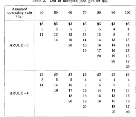
1. Our first attempt to demonstrate the rank ordering of the four different ARULE's got into trouble on the first data set because ARULE's 3 and 4 accepted the same jobs and accordingly provided exactly the same profits.

We used random number tables to determine all the data shown in Table 1. In job set #1, the one job with an impossible delivery commitment, is also the job with the smallest profit margin per ope-rating hour. Thus consideration of either profit margin or probability of meeting promise dates leads to the same job being assigned low

Table 3. List of accepted jobs (job·set #:2). Assumed operating rate 40 50 60 70 80 90 100 C%) #:3 #:3 #:3 #:3 #:3 #:3 #:3 5 5 5 5 5 4 4 14 13 13 13 13 5 5 14 16 14 14 13 13 ARULE=3 20 16 16 14 14 19 17 16 15 20 19 16 20 17 20 #:3 #3 #:3 #:3 #:3 #:3 #:3 5 5 5 4 4 4 4 14 14 16 5 5 5 5 _\ 16 17 15 14 14 14 I ARULE=4 15 I 18 16 15 15 20 19 16 16 16 i I 20 19 17

I

20 20 _._-.

(12)

priority.

In the second set of jobs, we can begin to see some differences in the priorities. Two additional jobs have impossible delivery promises. One of these, job #13, presents a very attractive profit margin. There are only 16 possible hours of work between the time when the order is accepted and the end of the promised shipping day. The job

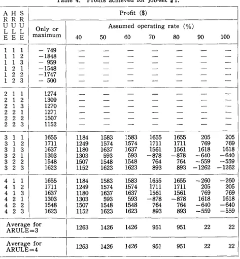
re-Table 4. Profits achieved for job·set # 1.

AHS Profit ($)

RRR ·

UUU _{Only or}

I

Assumed operating rate (%)

L L L E E E maximum 40 50 60 70 80 90 100 · 1 1 1 - 749 - - - -1 -1 2 -1848 - - -

-1 -1 3 - 959 - - -

-1 2 -1 -1548 - - - -1 2 2 -1747 - - -

-1 2 3 - 500 - - - -2 1 1 1274 - - - -

-

- -2 1 -2 1309 - - -

-

- - -2 1 3 1270 - - - -2 -2 1 1271 - - - -2 -2 -2 1507 - - - -2 -2 3 1152 - - - -· 3 1 1 1655 1184 1583 :~583 1655 1655 205 205 3 1 2 1711 1249 1574 1574 1711 1711 769 769 3 1 3 1637 1180 1637 1637 1561 1561 1618 1618 3 2 1 1303 1303 593 593 -878 -878 -640 -640 3 2 2 1548 1507 1548 1548 764 764 -559 -559 3 2 3 1623 1152 1623 1623 893 893 -1262 -1262 · 4 1 1 1655 1184 1583 1583 1655 1655 -260 -260 4 1 2 1711 1249 1574 1574 1711 1711 205 205 4 1 3 1637 1180 1637 1637 1561 1561 769 769 4 2 1 1303 1303 593 593 -878 -878 1618 1618 4 2 2 1548 1507 1548 1548 764 764 -640 -640 4 2 3 1623 1152 1623 1623 893 893 -559 -559 Average for

I

1263 1426 1426 951 951 22 22 ARULE=3 ·

I

Average for ₁₂₆₃ ₁₄₂₆ ₁₄₂₆ ₉₅₁ ₉₅₁ ₂₂ ₂₂ ARULE=4 ·

(13)

48 Kein08uke Ono and Curti8 H. Jone8

quires 20 hours of work. Table 3 shows the orders accepted under the two rules.

With the second set of jobs, our rank ordering of ARULE's received strong support. Tables 4 and 5 show the profits achieved by

various combinations of decision rules. Figure 1 summarizes the

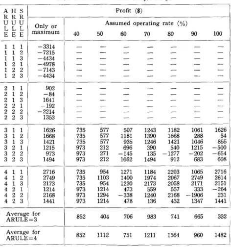
separate runs by showing the single or maximum value of net profit Table 5. Profits achieved for job-set # 2.

AHS Profit ($)

RRR

I

UUU _{Only or} Assumed operating rate (%)

0~H~1~1~1~2~2~2 __ -41~\~"li~/+l~\.2-+2~1+2 __ ~1_1~1~2~2~2~-41-4'-+'-+2-+2-+2~ \

:

I-~-2000 S w 1 2 3 I 2 3 1 ~ 3 ~I 213 1 2 3 I 2 3 1 2 3 1 2 3 \ I \I

~ 0 - - - 0 JOB - SET No. I a:

'"

I-'"

Z -4000 -6000

'1

\

\ f''rt

_, _I _\ _I

t

'I \

I , I \ I \ I \ I

K

Y

~ARULE JOB-SET---.. 2 t--~ JOB-SET No. 2

AVERAGE NET PROFIT ($)

2 3 4

-1386 1275 15BO 1580

-5391 254 1401 1966

_8000L-L-L-~~~ __ ~~~~~~ __ - L - L - L - L - L - L __ ~~~~~~

Fig. 1. Average profit rate for ARULE, HRULE, SRULE combinations.

for each triple rule combination (using whichever capacity assumption provided the best value). The highest profit shown on any of the ARULE=l runs is lower than the lowest profit on any of the others. ARULE=2 shows a lower profit on :5 of the 6 combinations than the most profitable assumed operating level for ARULE=3. On 3 of the 6 combinations, the ARULE=2 profit is more comparable to the worst assumed operating level. Using the profits achieved by the best assumed operating level, the profits of the ARULE=4 schedules are significantly better than the profits of the ARULE=3 schedul~s in 5, out of 6 combinations.

(15)

50 Keinosuke Ono and Gurtis H. Jones

more restricted set of choices in job set #1 to be more profitable than the abundance of choices presented in the order set #2. Only ARULE =4 has the power to distinguish among the choices so as to capitalize on the greater flexibility inherent in the larger data set.

We interpret these results to mean that the inclusion of consid-eration of the factors of profit, capacity and delivery in the acceptance process is extremely important in determining shop profitability. As the rules take more effective account of the interrelationships between individual orders and shop profitability, they have increasingly bene-ficial results. Our techniques of taking probability of lateness into account are particularly crude. We foresee an opportunity for the development of more sophisticated heuristic rules of order acceptance to match the development of heuristic scheduling rules.

1000

-

l- t i<: AI q 2 2 2 3 3 3 4 4 4 0 0 a: S t 2 3/ 1 2 3 2 3 2 3

'"

/

I-...

z 0--0 HRULE = t ~--l:. HRULE = 2 -1000

(16)

I-2000 A l l 1 2 2 /2 3 3 3 4 4 4 O~~~~~~-~~~~~~~ 5 I 2 3 I 2'3 I 2 3 I 2 3 1\ , I \ ,

,

\

,

\

,

K

i!5 -2000 It: 0.. I-IU Z -4000 -6000 0--0 SRULE = 1 ~--6 SRULE = 2 -8000L-L-L-L-L-L--L-L-~~~~~

Fig. 3. Effect of HRULE on profit (job-set ~2).

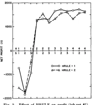
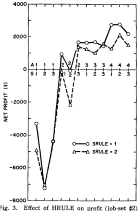
2. The raw data shown in Tables 4 and 5 and the lines shown in the graphic presentations in Figure 2 through 5 strongly support our contention of inconsistency. On the average, HRULE=2 provided less overtime and, in our relatively loaded shop, less profit, but there are many acceptance rule and scheduling rule combinations where HRULE=2 provided higher profits.

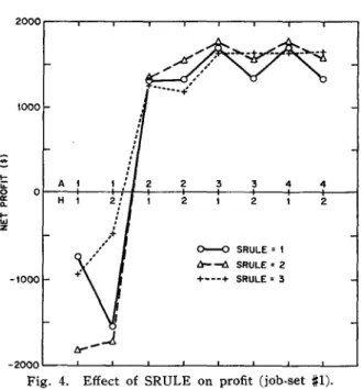
The relative rankings of the SRULE's are less clear. Figure 4 shows that each of the three SRULE's is the best with certain combi-nations of ARULE and HRULE in job set

#

1. With some of these combinations, the addition of the extra jobs in job set #2 changed the

(17)

52

- I-;;: 0 0:: a.. I-.... z

Keinosuke Ono and Curtis H. Jones

2000~--r---r---~--~--~--~--~--~--' 1000 A t 2 3 3 4 4 0 H

,

2 2 2 0--0 SRULE' t 6---.l. SRULE' 2 -1000 + .. --+ SRULE' 3 -2000 L--._'--__ ' - -__ -'--__ -'--__ -'--__ -'--__ . J -_ _ -'---l Fig. 4. Effect of SRULE on profit (job.set #1).

relative ran kings of the three SRULE's. Figure 5 shows the shifts in relative SRULE rankings associated with small changes in the operating level.

Our explanation of the inconsistency is still that the HRULE's and SRULE's we have included are gross oversimplifications of the interrelationships between overtime and scheduling decisions and final profit. The way the jobs and overtime drop into place are too com-plicated to be governed by the continued application of some simple rule. This could be construed as supporting evidence for the Ferguson and Jones contention that the way to help schedulers is to get them to work with more different alternative schedules rather than to try to devise the best set of decision rules.

I tr-.J. -8000~~--~--L-~----L--~~~-L~

Fig. 5. Effect of SRULE on profit (job-set #2).

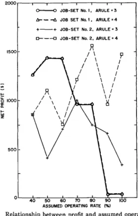
would be very zig-zagged. Even when these figures are aggregated and averaged in Figure 6, there is very is limited evidence of any smooth curve.

One possible explanation of the erratic and unpredictable nature of these profit figures is that they are caused by our unrealistic short-term measurement of profit. We examined this possibility by adjust-ing the profit figure to give credit proportional to the hours of work accomplished. Table 6 shows the adjusted profit for various' SRULE and HRULE combinations with ARULE's 3 and 4.

(19)

54

I-Keinosuke Ono and Curtis H. Jones

1500·

0 - - - 0 JOB·SET No. I, ARULE' 3

~ - -A JOB SET No. I, ARULE = 4

+ - - + JOB-SET No. 2, ARULE' 3

cr---o JOB-SET No. 2, ARULE = 4

,R / \ 71 / \ I / \ / / \

P

\ /

\ I \ I ~ 1000 g:: \ I

g

I-'"

Z 500 0L-~40~~50~~6~0--~ro~~80~~9~0--~--~

ASSUMED OPERATING RATE (%l

Fig. 6. Relationship between profit and assumed operating rate under ARULE=3 and ARULE=4.

Note: These data are the averages of the various HRULE and SRULE combinations for the ARULE and operating rate shown here.

profit figures but they can still not be considered to be members of a family of unimodal curves. The reader should notice such anomalies as the profit figure for the combination of ARULE=4, HRULE=2, SRULE=2, and an assumed operating rate of 90%.

After examining these figures, we wondered about the relation-ship of actual operating rate to assumed operating rate. The erratic

(20)

Table 6. Adjusted profit for job·set ~2.

AHS Profit ($)

RRR

Maximum

I

UUU Assumed operating rate (%)

L L L EEE 40 50 130 70 80 3 1 1

I

2134 3 1 2 1668 3 1 3 1778 3 2 1 1551 3 2 2 I 973 3 2 3 1608 4 1 1 2716 4 1 2 2749 4 1 3 2536 4 2 1 1292 4 2 2 2168 4 2 3 1949 Average for I ARULE=3 Average for I ARULE=4 80 70 - 60 .,t ~ 50

'"

C) z ~40

'"

a. 0 ..J 30 C( :::> .... u C( 20 0 10 735 577 507 735 577 Ll81 735 577 935 973 627 819 973 686 595 973 627 1062 735 954 1271 735 1103 1400 735 954 1220 973 1214 798 973 1294 377 973 1214 803 854 612 840 854 1122 978 /:; /:; 0 0 ~ 0 /:; 1243 1422 1390 1668 1246 1421 1244 ll05 969 184 1494 1510 1484 2203 1974 2067 2173 2058 1184 1297 1565 2168 946 1151 1261 1218 1554 1807 o O-ARULE' 3 /:;-ARULE' 4 OL-~4~O--~5~O~-6~O~-=roO--~80~~9~O--~IO~O~~

ASSUMED OPERATING RATE (%)

90 100 1501 2134 738 829 1467 1778 1551 638 573 157 1608 1275 1609 2716 2749 2614 2356 2334 739 913 10 1006 1857 1949 1240 1135 1720 1922

(21)

56 1500 ~ 1000 >-.: o et: 0- >-W Z 500

Kein08uke Ono and Curti8 H. Jone8

+ + ,,/" .."

--" + +

"

I I I I 0 I + / / / + I • I 0

/

0 - - 0 ARULE • 3 +--+ ARULE' 4 %~--1~0--~2~0--~3~0--~4~0--~5~0--~6~0--~7~0--~80

ACTUAL OPERATING RATE (%)

Fig. 8. Relationship between adjusted profit and actual operating rate in job·set #2.

nature here can be presumed due to the bunching of work at certain machines at certain times in the schedule.

Figure 8 shows a graph of adjusted profit against actual operat-ing rate. We have drawn approximatoperat-ing smooth curves for the two ARULE's. It appears that both lines are flattening out as higher operating rates are allowed. The ARULE=3 line suggests that with this cost structure and environment, attempts to load the shop to more than the 50% level will cause decreasing profits. Because the ARULE=4 policy considers more of the channels through which ac-ceptance decisions affect profit, it is able to take better advantage of the physical facilities. It continues to provide increasing profits at

(22)

an actual operating rate of 60%. Summary

The shaping of acceptance rules to take more effective and com-plete consideration of the ways the introduction of a particular order will affect the profits of a job has been demonstrated clearly to be an important task. More complete consideration of the factors pro-duces significantly higher profits.

Present heuristic rules for order acceptance, overtime and se-quencing are far from optimizing. Various combinations of inputs and rules react in ways which can only be evaluated by simulation. Under these circumstances, it would seem very useful to design systems which allow the decision maker to consider alternative rules.

The primary connection between the order acceptance policy and the profit of a job shop would seem to be through the average operat-ing rate. Yet when we attempted to accept the best set of jobs to fit a range of assumed operating rates, we were unable to find a regular, predictable relationship between profit and the assumed operating rate. The development of effective production management decision making systems demands an increased understanding of this relationship. Further simulations with more complex cost structures, including the effect on future demand and with a broader range of heuristic rules, will be required to establish some guidelines to help managers find the acceptance policies best suited to their cost struc-tures. We believe simulation in this area will be more productive than more simulation in dispatching rules.

This work has treated order rejection as a feasible alternative. Many firms do not appear to have this choice. We believe that the establishment of realistic promise dates which take into account the long-term effects of displeasing this customer, of possible delays on other orders, and of the available capacity can be formulated as a

(23)

problem amenable to decision rules. The promise date rules should be simple heuristic rules attempting to take into account the various factors we have identified.

References

[1] Conway, R.W. and W.L. Maxwell, "Network Dispatching by the Shortest Operating Discipline," Operations Research, 10 (1962).

[2] Conway, R. W., W. L. Maxwell and L. W. Miller, Theory of Scheduling, Reading, Mass., Addison·Wesley, 1967.

[ 3] Ferguson, Robert L. and Curtis H. Jones, "A Computer Aided Decision System," Management Science, June (1969).

[4] Gere, William S., "Heuristics in Job Shop Scheduling," Management Science, November (1966).

[5] Holstein, WiIliam K., "Production Planning and Control Integrated," Har-vard Business Review, May·June (1968).

[6] Jackson, J. R., "Some Problems in Queueing with Dynamic Priorities," Naval Research Logistics Quarterly, 7 (1960).

[7] Jones, C. H., J. L. Hughes and K. J. Engvold, "A Comparative Study of Computer· Aided Decision Making from Display and Typewriter Terminals," IBM Technical Report, TR 00.1891, June, 1969.

[8] Rowe, Alan J., "Toward a Theory of Scheduling," Journal of Industrial Engineering, 11, Mar.-Apr. (1960).

[9] Senju, Shizuo and Y. Toyoda, .. An Approach to Linear Programming with