AN EXACT AGGREGATION FOR INVENTORY DISTRIBUTION IN AN AUTOMATIC WAREHOUSING SYSTEM

Vol. 41, No. 4, December 1998

A N EXACT AGGREGATION FOR INVENTORY DISTRIBUTION IN A N AUTOMATIC WAREHOUSING SYSTEM

Hideaki Yamashita Hiroshi Ohtani Shigemichi Suzuki Tohoku University NEC Corporation Chiba Institute of Technology

(Received September 26, 1996; Revised September 24, 1997)

Abstract We consider a simple automatic warehousing sytem with a lot of storage spaces called slots in which only a single type of items are stored and retrieved. The purpose of this paper is to develop an efficient method for obtaining the marginal probability that each of the slots in the warehouse is full. The set of such probabilities for all the slots constitutes the spatial inventory distribution of the items in the system. This distribution, which we call the inventory distribution in short, enables us to evaluate key performance characteristics of the system such as the mean travel time of a crane for a single operation of storage or retrieval of items. Such characteristics cannot be obtained from the distribution of the total number of full slots alone.

We assume that inventories are controlled by an (S, S) reordering policy, and that received items are

stored from the closest open slot to an 110 point and retrieved items are chosen randomly among currently full slots. Furthermore the time between retrievals and the time between placing of order and receipt of items are exponentially distributed. Under these assumptions the system can be modeled as a Markov chain. If we use joint inventory levels of slots, the number of states of the Markov chain amounts t o 2m, where m is the total number of slots. Here we devise exact aggregation methods of the states to reduce the size of the Markov chain. By exploiting the special structure the total computational complexity for obtaining the inventory distribution is reduced to 0 ( m 4 ) .

1. Introduction

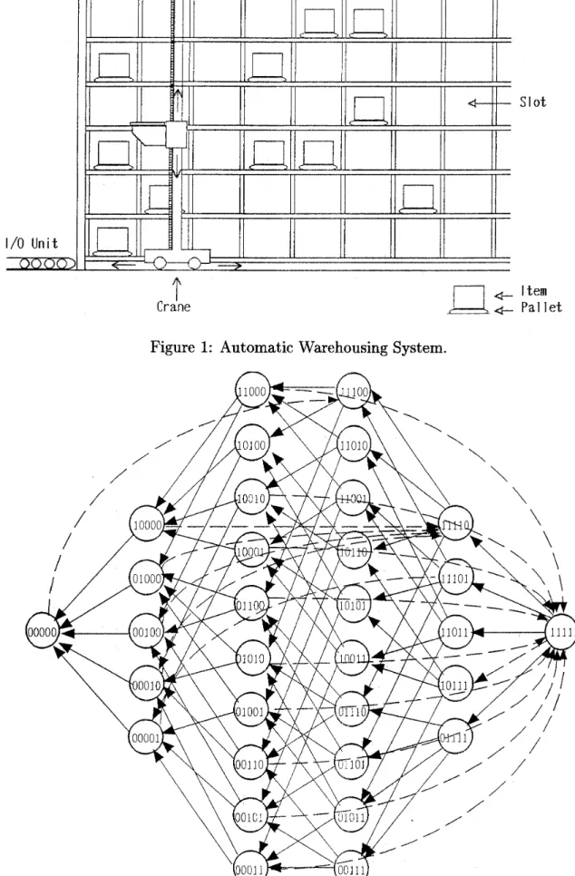
A typical automatic warehousing system has, among other things, racks with slots in which items are stored, a stacker crane which stores and retrieves items automatically, and a computer which controls the operations of the crane and the inventories as shown in Fig. 1. An order for items is placed according to a certain inventory policy. When items arrive at

the warehousing system, they are assigned to pallets and then the pallets are put into the system from the 110 point. In the warehousing system items are controlled in the unit of pallet. The crane transports each pallet from the 110 point to one of open slots, and stores it in the slot. Retrieval of items will be done almost in the reverse order.

The computer chooses a slot for storing or retrieving according to a certain rule. This rule as well as the inventory control policy based on assumptions on request for retrieval of items and delivery lags has a great influence upon the performace of the warehousing system. As we will show in Section 2.3 the distribution of the total number of items in the warehouse can be obtained rather easily. However, this is not sufficient to evaluate such key performance characteristics as the mean travel time of the crane for an operation of storage or retrieval of items. We must know also how items are distributed in the system with respect to the 110 point. We will consider the marginal probability that each slot is full, then the set of such probabilities for all the slots in the warehouse will constitute the spatial inventory distribution of the items in the system. We call this spatial distribution as the inventory distribution in short. Once the inventory distribution is known, the distribution of

An Aggregation for Inventory Distribution 493

travel time can be determined from the geometrical configuration of slots in the warehouse and the physical performance of the crane such as speed and load/unload time of items. The distribution of traveling time is a key operating factor for evaluation of overall warehousing systems, though for that purpose such performance characteristics as queue lengths of pallets of items yet to be stored into slots and unfilled requests for retrieval of items must be also taken into account. The overall evalution of warehousing system requires a comprehensive model-building process and will be a topic of for further research. In this paper we will devote ourselves to determination of the inventory distribution in the warehousing system operated by (s,S) policy in order to estimate the travel time distribution. Although the inventory distribution is very important in designing warehousing systems, all of the previous works on the related topics have not treated the inventory distribution adequately. In this paper we will show that the inventory distribution can be obtained with reasonable computational efforts by aggregation methods.

In some previous works analytical expressions are obtained for travel time of a crane in automatic warehousing systems. Based on the expected travel times of the crane, Hausman, Schwarz and Graves [4] compared three storage methods, i.e., randomized storage, turn-over based storage and class-based storage. Another paper by Graves, Hausman and Schwarz[3] investigated analytical and empirical results for various combinations of alternative storage assignment rules and interleaving rules. In [4] and [3], they have assumed that the 110 point is located at the corner of the rack and that the rack is square in time, i.e., the crane can get to the remotest point from the 110 point in the vertical direction and such point in the horizontal direction in the same length of time. Bozer and White [l] determined the expected travel time for alternative the

110

point locations and rack configurations. Hwang and Lee [2] and Chang et al. [5] further generalized the previous models by considering the acceleration and deceleration rates of an SIR machine. In these analyses an assumption is made that items are stored in the rack uniformly. This assumption makes the analysis easy. In real systems, however, this is not the case. There are open as well as full slots, and the distribution of full slots is not uniform. The assumption of uniformity gives rise to noticable errors. Thus the purpose of this paper is to establish an efficient method for obtaining the inventory distribution t o evaluate warehousing system more accurately.

Noguchi and Suzuki [7] have taken into consideration the inventory distribution in an-

alyzing the automatic warehousing system. In their system, n different types of items were assumed to exist and inventories were controlled by an ( S , S) reordering policy. They

supposed that received items were stored from the closest open slot to the 110 point and retrieval was random among the same type of items. Under further assumptions of random arrival and random request for items this system can be formulated as a Markov chain with (1

+

nlm states, where n and m are the numbers of item types and the slots respectively. It is almost impossible for practical sizes of m and n to solve the system of equilibrium equations for the steady state probabilities. Then they proposed an approximate solution method for this problem.

In this paper we employ the same model as in [7] but restrict ourselves to a single type of items. Then we show that aggregation leads us to a smaller Markov chain which provides us the inventory distribution with less computational efforts. More specifically we focus our attention on whether slot i (i = 1,2,

.

,

m) is full, the total number of full slots, the number of full slots among first z slots, and associated states, then we can get an aggregated Markov chain whose transition probabilities are all known. Although the model will have 2m states if we use joint inventory levels of slots, the aggregation reduces the number of states to 0(m2) for each slot. In addition, we propose 0 ( m 3 ) time algorithm for obtaining

S l o t

T

+, item

Crane +. Pallet

Figure 1 : Automatic Warehousing System.

An Aggregation for Inventory Distribution 495

the steady state probabilities of the aggregated states by utilizing the structure of the linear equilibrium equations for each slot. As a result, our algorithm makes it possible to obtain the inventory distribution for all the slots in 0(m4) time. This gives a way t o analyze the inventory distribution in an automatic warehousing system with a practical number of slots. In Section 2 we will describe our model and assumptions and make preliminary analyses about the probability distribution of the total number of full slots and equilibrium equations for joint inventory levels of slots. There are two types of aggregation depending on the location of slots. In Sections 3 and 4 we will show those two aggregation methods and efficient methods for solving the aggregated systems of equilibrium equations respectively. Section 5 contains results of numerical experiments and Section 6 gives concluding remarks and comments on extensions.

2. Model and Preliminary Analysis

2.1. Assumptions and Notations

The assumptions and notations in our model will be described in the following:

(a) Only a single type of items are treated in our model. The quantity of items is counted in the number of pallets.

(b) There are rn slots in the automatic warehousing system. To make the argument simple, the slots are assumed to be in a row and numbered from 1 (the closest slot to the 1/0 point) to m (the remotest slot from the I/O point).

( c ) Each slot can store one pallet of items.

(d) Requests for retrieving one pallet come to this system according to a Poisson process with a constant rate p. When a request for retrieval comes, the items on a pallet are taken out from one of the full slots which is chosen at random. If there are no items in the system at that time, the request is lost.

( e ) The inventory is controlled by an (S, S) reordering policy, i.e., if the inventory level

decreases to r (reordering point), a reorder of q (reordering quantity) pallets of items will be placed, where r and q are prescribed constants. The lead time between placing of order and receipt of items is exponentially distributed with a constant parameter A.

(f) As soon as q pallets of ordered items arrive at the system, each pallet is stored in the closest open slot to the 110 point.

( g ) The number of slots is equal to the maximum inventory level, i.e., m = r

+

q. The reordering point is less than the reordering quantity, i.e., r

<

q.

(h) The time required for storage or retrieval of pallets which consists of the travel time of the crane and the load/unload time of items at the 110 point and the slots is assumed to be zero, so we can neglect the waiting time for the crane.

Some of the assumtions will be explained to clarify our standing point: Storing of each pallet of arriving items in the closest open slot to 1 / 0 point (assumtion(f)) is natural since it makes the travel time short. A pallet of requested items are assumed to be taken out at random from one of the full slots (assumption(c)). There are alternatives for this rule: One rule is of taking out a pallet from the slot to the closest to 110 point and another is of taking the oldest pallet in the warehouse. Those rules may either leave very old items in the warhouse or require history of inventories in the warehouse and time-consuming processing. A rule of assmption(c) is simple to operate and does not leave old items excessively. It may seem contradictory to neglect waiting time of the crane since we are interested in travel time of the crane. Remember that we are going to determine the inventory distribution in

the warehouse. If arrivals of ordered items and requests for retrievals of items are processed in FCFS (First Come First Served) basis,the inventory distribution of items at a moment of start of storage or retrieval of pallets does not depend on time required for storage or retrieval of pallets. This permits us to set time required for storage or retrieval arbitrarily. Hence as far as the inventory distribution is concened we can neglect the time required for movement of the crane and processing of pallets. Of course the time associated with crane must be taken into account to evaluate the overall performance of the warehousing system.

2.2. Probability Distribution of Total Number of Full Slots

Let X(t) be a random variable designating the total number of full slots in the warehouse at time t. From the assumptions on Poisson arrival of ordered items and random request for retrieval of items described in Section 2.1 the stochatic process X(t) is ergodic and Markovian. Let P(i) be the steady state probability that X(t) =

i

(i = 0,1, a

,

m). The

system of equilibrium equations for P(i) can be easily obtained as follows:

I

AP(0) = ) #(l/. (2 = O),

(A

+

p)P(i) = pP(i

+

l) (1

5

S

r), ,uP(i) = p P ( i

+

l) (r

<

2 q),

pP(2) = \P(i

-

q)

+

p P ( i

+

l) (q

5

2 < m ) ,

pP(m) = W ( r ) (i = m).

After a little algebra, we can express P(i)'s only with P(q) as follows: (i =

O),

by using these equations and the condition

we can get P ( q ) at first, and other P(z)'s can be obtained by (2.1) easily. Those probabilities along with other more detailed information will be used in Section 3.2 to compute the inventory distribution, i.e., the probability that each of the slot is full.

2.3. System of Equilibrium Equations for Joint Inventory Levels for Slot 1 to m

Let Xi(t) be a zero-one random variable denoting whether slot i is full (1) or empty (0) at time t and xi be a value which Xi(t) assumes (i = 1,2,

-

,

m). It is easy to see from the assumptions described in Section 2.1 that the stochastic process {(Xl (t)

,

X2

( t )

, ,

Xm (t))} is ergodic and Markovian. Let P(xl, xi,

-

,

xm) be the stationary joint probability for inventory levels for slot 1 through slot m

,

namely,

We assume that P(xi, x i , .

,

xm) = 0 for impossible states, i.e., the states for which some

xi is neither 0 nor 1. The system of equilibrium equations for the warehousing system can be written down referring to, for example, Fig. 2 in case of m=5, q=3, and r=2. The equations

An Aggregation for Inventory Distribution

are of different forms depending on the total inventory level as follows:

where

and ei (i = 1 , 2 , - - - , m ) is either 0 or 1.

We will briefly explain the equilibrium equations (2.2). For 1

5

f m

5

r , both an arrival of ordered items and a request for retrieval cause trantiotion out of the state (xi, x2,

,

xm}

with the rates \p and pp respectively, where p is the stationary probability of designated state. In addition, transitions from (m - fm) states with the inventory level fm

+

1 into the state (X\, x2,

,

xm) will occur due to a request for retrieval with the rates pi/(fm

+

1)

since the pallet is retrieved at random among (fm

+

1) full slots. For r

<

fm

<

q, no transitions occur associated with arrival of ordered items. The transition rate out of the state (x1

,

x2,

,

xm) is pip and transitions from the states with the inventory level fm

+

1 into the state ( x l , x 2 , - - - , x m ) are the same as the case 1

<

f m

<

r . For q

<

fm

<

m the situation is the same as in the case r

<

fm

<

q except that there exist transitions from the states with the inventory level (fm - q) into the state (xi, x2,

-

-

,

xm) due to arrival of ordered items with the rate \p. For For q

<,

f m

<

m, we have expressed the situation concretely that q arriving pallets have been put into empty slots up to slot m. The case fm = m is the same as the case q

<

fm

<

m except that there is no transition into the state (xi, x2,

,

xm) due to retrieval of items.

The system of equilibrium equations has 2m unknown variables. If we can solve it, we, of course, obtain the marginal probabilities by

But it is practically impossible, because real systems have more than thousand slots in some cases. Therefore we need some devices to overcome this difficulty.

3. Exact Aggregation Method I

3.1. Aggregation for Slots 1 to q, and m

In this section and next, we will propose an exact aggregation method for the inventory distribution, i.e., the probability that each of the m slots in the warehouse is full. This method does not give the probabilities for all the slots at the same time, but gives the probability for each slot individually. We will reduce the computation time drastically by aggregating associated states of the Markov process so as to keep the necessary information for obtaining the probability that the slot is full. We use two kinds of aggregation depending on which slots we are working on: The one is for obtaining the probability that each of slots

1 q and m is full and the other is for the rest of the slots. In this section, we will explain the former.

Our purpose is to establish an efficient method for computing the marginal probability

P r ( X i ( t ) = l ) ( i = l ,

-

- , m ) .

Let F,(t) be a random variable designating the total number of full slots in slot 1 through

and let fi be a value which Fi ( t ) assumes. We will introduce a stochastic process { ( X i (t )

,

Fm ( t ) ) } with 2m states for each i to reduce the number of states of the original Markov process. Note that there do not exist states ( 1 , O ) and (0, m ) for each i. Associated with each of 2m states (xi,

fã

define a set Si(xi, f m ) as

then

k=O k=l

will be a partition of the set S of all the 2m states of the original Markov process. There exists

a one-to-one correspondence between a state ( x i , f m ) of the stochastic process { ( X i (t )

,

Fm ( t ) ) } and a set Si(xi1 f m ) of states of the original Markov process.

The stochastic process { ( X i ( t ) , Fm(t))} is also a Markov process for 1

5

i

<

q and z = m.

In order to show this, first define the transition rate from a state X = ( x i , X ^ ,

,

X ~ ) E S ~ ( X ~ ~ f m ) to a set of states &(xi,

fh)

based on the transition rate p(x, X ' ) from a state X to a state

X' = (X',

,

X , ,

-

,

X') of the original process as

Essentially due to the lumpability theorem of a Markov chain of Kemeny and Snell [4, p.1241, the stochastic process { ( X i ( t ) , F m ( t ) ) } is a Markov process if and only if for every pair of sets Si(xi,fm) and Si(xi1

fh)

,

p(x, Si(x',, f ; ) ) has the same value for every x&Si(xi, f m )

This common value will be the transition rate from a set of aggregated states Si(xi, f m ) to another set Si ( x i ,

fã

or equivalently from a state (xn f m ) to a state ( X ; f;) of the stochastic

process { ( X i

(t),

Fm ( t ) )

}

Now we will show that p(x, Si(x<,

fh))

has the same value for every x&Si(xi1 f m ) - Con- sider a state x&Si(xi, f m ) and the set of states S, to which transitions are possible in one step caused by retrieval or receipt of items from X . If fm

<

r receipt is possible and S, has a single element X' and the rate of transition is A since received items are stored from the

closest open slot to the 110 point (see assumption (f)). In case of i

<

q, x1&Si(l1 fm

+

q ) is

the only state after receipt of items for any x&Si(xi, f m ) , but for m

>

i

>

q there exist y'

and z' such that

yl&Si(O,fm+q) and z1&Si(l1fm+<f)

are the states right after receipt of items. This means that the transition rate p ( x , S , (0, f m

+

q ) ) does not necessarily have the same value for every xeSi(O, fm}. This implies that the stochastic process { ( X i (t )

,

Fm ( t ) ) } is not Markovian if m

>

i

>

q, but it will be Markovian if

i

<:

q and the transition rate defined in (3.1) has a common value for transitions by retrieval

An Aggregation for Inventory Distribution 499

Now we will consider transitions caused by retrieval of items. If fm

#

0,

retrieval is possible and items in one of full slots will be taken out a t random. There are fm states in

Sx

in this case. We will consider two sub-cases, i.e., the cases Xi =

0

and

xi

=

1.

In the former case all the possible transitions are into one of the states in

Si(O,

fm

-

1)

and

for all

xeSi(O,

fm)

because of Assumption (d). In the latter case two kinds of transitions are possible: One is a transition into one of the states in

Si(O,

fm

-

1)

and the other is a transition into one of the states in

Si(l,

fm

-

1).

Because of Assumption (d) again, we have

P(X,

Si(0,

fm -

1))

= p/ fm and p(%,

&(l, fm

-

1))

= (fm -

1)p,/fm

for all

x&Si(l,

fm).

We have shown that the transition rate

(3.1)

has a common value for every

xeSi(xi,

fm)

for transitions by retrieval of items. The discussions above now have established that the stochastic process

{(Xi((),

Fm(t))}

is a Markov process if >'

5

q. We denote by

Pi(,xi,

fm)

the steady state joint probability distribution for the inventory level of slot i and the inventory level of the system. Then we can derive the system of equilibrium equations for

fi(xi,

fm).

There is, of course, one equation for each state

(xi,

fm).

The equilibrium equations for

Pl(xl,

fm)

are derived as a typical example in the following by classifying them with the value of

fm.

The system of equations are written down in the following in the descending order of

fm

since those equtions are referred to in this order later in this paper:

'

APi(0,

r)

+

APl(1,

r) -

p,Pl(l,

m) =

o

(fm =

m),

APl(0,

fm - q)

+

APl(1,

fro - q)

+a(fm)~Pl(l,

fm

+

1)

-

pPl(1,

fro) =

0

(q

<

fm

<

m),

a(fm)~Pl(l,

fm

+

1)

-

/^Pl(l,

fm)

=

O

(r

<

fm

<

4,

a(fm)Fi(l,

fm

+

1)

- ( p

+

A)Pl(l,

fm) =

o

(l

5

fm

<

r),

b(fm)/^l(l,

fm

+

1)

+

/^P1

(0,

fm

+

1)

-/^Pl(O,

fm) =

0

_(r

<

fm

< m ) ,

b(fm)~Pl(l,

fã

+

l)

+

pp1 (0,

fm

+

1)

-(P

+

A)Pi(o,

fm) =

0

(1

5

fm

5

r),

/iPi(O,

1)

+

/iPi(l,

1)

-

APl(O,

0)

=

0

(fm

=

O),

K 2 0

^(O,

fm)

+

27n=i

Pl(1,

fm)

- l =

0,

Since the state tranisitions in the aggregated Markov process are similar to those in the original process explained in detail in Section

2.3,

we will explain only the case q

<

fm

<

m

here. Transitions into state

(1,

fm)

by receipt of items are from states (0,

fm

-

q) and

(1,

fm - q) respectively both with transition rate

A

which correspond to the first and the second terms. A transition into state

(1,

fm)

by retrieval is from state

(1,

fm

+

1)

with the rate

p((1,

fm

+

l),

(1,

fm))

=

fml^/(fm

+

1)

=

a(fm)/'

which corresponds to the third term. A transition out of this state

(1,

fm} is possible only by retrieval of items. The transition rate is p, from

(3.2)

which corresponds to the last term. We will show an example of the aggregation for the model with m = 5, q = 3, and r = 2. The state transition diagram of the system before aggregation is shown in Fig. 2 which corresponds to the equilibrium equations

(2.2).

After aggregation the state transition diagram for the states

(xi,

fm)

will

be as shown in Fig. 3 which corresponds to the first seven equations of (3.3). In general the state transition diagram for the states ( x i , fm) will be as shown in Fig. 4. (3.3) is a system of linear equilibrium equations with 2m unknown variables. The number of variables is much less than that in (2.2).

Among m variables X i ( t )

,

a

,

X m

( t )

,

q variables X i

( t )

,

-

,

X ,

( t )

are the random vari- ables which have the same characteristic as

Xi(^).

We can apply the same aggregation method as above to each of slots 2 q and exactly the same system of equilibrium equa- tions as (3.3) can be obtained for

PAX^

fm) for each 2 . This means that the probability that

slot 2 is full is the same for i = 1 , 2 , *

-

,

q. We can see it intuitively because of the rules

for storage and retrieval in Section 2.1. The states of slot m can be described similarly to those of slots 2 through q and the same type of aggregation can be applied. The system of equilibrium equations for Pm(xm, f m ) is as follows:

which is also a system of linear equilibrium equations with 2rn unknown variables.

3.2. Solution Method for P ( X i ( t ) = 1) ( 2 = 1 q and m)

Systems of equations (3.3) and (3.4) both have 2 m unknowns. These equations can be solved with any of standard methods for a system of linear equations. But we will develop a more efficient method by making use of the special structure of the equations. Once P i ( l , fm)'s are known the marginal probability that each of slots 1 q and rn is full can be obtained

m

P T ( X i ( t ) = 1 ) = Pi ( l , fm) ( 2 = 1 q and m ) . (3.5) fm=l

Now we will present a method for solving Equations (3.3) and (3.4). This method will use the distribution P ( i ) of the total number of full slots described in Section 2.2. For this purpose we will transform the first four equations of (3.3) as follows observing that

An Aggregation for Inventory Distribution

Figure 3: State Transition Diagram for States

(xi,

f m ) (m = 5, q = 3, r = 2).

NOW

Pi

( l , fm), fm = m, m - 1,

.

-

, l , are obtained recursively. Similarly, we can transform the first four equations of (3.4) to

. .

A j P

Pm(!, q

+

1) = [(q

+

l)/(! - -

E;;;

--(-)'-^+l

P q + j \ + P )/mlP(m)7

The third and fourth equations of (3.6) are obtained from the fourth and third equations of (3.4), respectively. The rest of the equations of (3.6) are derived by substituting those equations into the second equation of (3.4). We can obtain Pm ( l , fm) ( fm = l

,

,

m) from

(3.6).

Now we can obtain &(l, fm) (fm = 1,

,

m) for z = 1,

,

q and m with much less effort than solving (3.3) and (3.4) by standard numerical methods such as Gaussian elimination method. The computational complexities for solving them are dominated by those for obtaining fi(xi, fm) for 2 = q

+

l

-

m - 1 as we will see in Section 4.2.

4. Exact Aggregation Method I1

4.1. Aggregation for Slots q + l to m - 1

Exact aggregation of 2rn states S of the original Markov process into 2m states Si(xi7

fd

was successful to obtain Pr(Xi(t) = 1) for i = 1, 2,

,

q, and m. The Markov process thus obtained was {(Xi (t), Fm(t))}. This kind of aggregation will fail for à = q+ 1, q+2,

,

m- l . The reason for this was briefly explained in Section 3.1. We will examine the situation again and propose another method of exact aggregation which enables us to compute P r ( X d t ) =

1) for i = q + 1 , q + 2 , - - . , m - 1.

Suppose that q

<

z

<

m, f m

<:

r, and Xi(t) = 0, then receipt of items is possible in the state (0, fm) in the Markov process {(Xi(t), Fm(t))}. On receipt of items a transition occurs and the new state will be (1, f m

+

q) if fi

>

i - q and (0, fm

+

q) if fi

<

2 - q. The lumpability condition fails to hold for such a case since the state does not have information on Fi(t)

.

We need more information to get Pr

(Xi

(t) = 1) for i = q

+

1, q

+

2,

,

m - 1. To overcome the difficulty we will introduce a stochastic process

{(4

(t)

,

Fm (t))} or equivalently {

(&(t),

Gi

(t)))

where Gi(t) is a random variable defined by

The number of states of the stochastic process is less than (m2

+

4m

+

4)/4 (since K ( t ) and Gi(t) have (i

+

1) amd (m - i

+

1) states respectively) which is still much smaller than that of the original Markov process.

We will show that the stochastic process {(Fi (t), Gi (t))} is Markovian almost in the same way as we proved that {(Xi(t), F d t ) ) } was so. First we will define the sets of states by

An Aggregation for Inventory Distribution ₅₀₃

where gi is a value which G i ( t ) assumes. All the sets T , ( f i , gi) for each

i

clearly constitutes a partition of S. Define the transition rate from a state x & T , ( f i , gi) to a set of states T , ( f i 7 g:)

If we can show that for every pair of sets T,( fi, g,) and T , ( f < , g;), the transition rate has the same value for every x & Z ( f i , g i ) , then an aggregated Markov process can be constructed. This common value forms the transition rate from an aggregated state T , ( f i , g i ) to another

( f : , g:) of the aggregated Markov process or equivalently from a state ( f i , gz) to another state

( f i ,

g;) of the Markov process { ( F i ( t ) , G i ( t ) ) } .

We will show that the transition rate defined by ( 4 . 1 ) actually has a common value. First let xeT,[fi, 9,). If fi

+

g,(= fm)

-

<

r , then a transition from X due to receipt of items is possible with the rate A. Every possible state of the original Markov process after this transition belongs t o the state

G(/.,

g:)

,

where

and the transition rate in ( 4 . 1 ) has the same value A for every x & 3 ( f i , gi}.

If fi

+

gi{= f m )

#

0 , then transitions from a state X&% ( f i , gi) due to retrieval of items are possible into states in

z(fi

- 1 , gi) and Ti{f^ gi - 1 ) whose transition rates

are the same for every x & 5 ( f i 7 gi) and the sum is equal to p.

From the above discussion the stochastic process { ( F i

( t ) ,

G,

( t ) ) }

has been proved to be Markovian. We will denote by ( f i , gi) the stesdy state joint probabilities for the inventory level of slots 1 i and that of slots i

+

1 N m. Then we can derive the system of equilibrium

equations for

c(

f i , g i ) using the transition rates obtained above. It will be as follows:

where

= ( f i

+

l ) / ( f m

+

l ) , tGm = (gi + l ) , ( f m + l),

and P/(*, *)'S are assumed to be zero for undefined states. The state transition diagram for the states ( f f

,

g^) is shown in Fig. 5 . Since each of the equations of (4.5.1) (4.5.6) can be derived in almost the same way, we will explain only the first equation which is for fi = i. We will consider the transitions into state ( i , g,) as well as the transitions from the state. The transitions into state ( i , gi) are possible by both retrieval and receipt of items. Since the

first z slots are full after transition, retrieval must be from one of the slots i

+

1, i

+

2,

,

m.

This means that a transition is from state ( fi, gi

+

l ) of the aggregated Markov process whose transition rate is tifm = (gi

+

l)/( f m

+

l) from the second equation of (4.4) which correspond to the first term. The transitions into state

(i,

gi) due to receipt of items are possible from a set of aggregated states, i.e.,(; - q

+

gi, O ) , (z - q

+

g,

+

1, l ),

,

(z

-

q

+

1, g,

-

l), and 1

-

q,gi) acccording to equations (4.2) and (4.3). Then we will get the second term of (4.5.1) because each transition rate is A. Since i

>

q, transitions from the state are possible only by retrieval of items and the sum of these transition rates is p as was observed above which corresponds to the last term.

i - q

An Aggregation for Inventory Distribution

4.2. Solution Method for Pr(Xi(t) = l ) ( i = q + l , - - - , m - 1 )

If the solution of the system of equilibrium equations (4.5.1) W (4.5.6) is obtained, we can

get the expectation of

4

by

Then we can obtain the marginal probability that slot i is full by

whereE[Fq] can be obtained by

Pr (X1 (t) = 1) is, of course, obtained by (3.5) after solving Equations (3.3) using the method explained in Section 3.3.

(4.5.1) --' (4.5.6) is a system of linear equilibrium equations with 0 ( m 2 ) unknown vari-

ables: More precisely the number is less than (m2+4m+4)/4. Now, let us show an algorithm for solving it in 0(m3) time by utilizing its structure. First we will reduce the number of variables to m - i

+

2 by expressing each of P'Afz, gi) (

fi

= 0,

-

,

i, gi = 0 , . . - , m à ‘ i as a

ofe1(q,k) (k = 0 , - - - , m - i), i.e., linear combination

where obviously

holds and the rest

(g, = k),

c q , g i , k = 0 (otherwise )

,

(k = 0 , 1 , - S - , m - i )

of the coefficients are obtained recursively to be explained below. To simplify the notation, we use Cf^ instead of Cfi,gi,k, a and t instead of and The coefficient Cigk can be obtained from (4.5.1) W (4.5.5) as follows: First suppose that Pl(q, k)

(k = 0,

,

m - i) are known for the time being, then q f ( q - 1, gi) can be expressed in terms of P[(q, gi) using (4.5.3) for gi = m - i, m - i - 1, , 0 and the coefficients will be be obtained as in (4.10.1). The same relation holds for r

<

f

+

g and f

<

q. The coefficients are obatined in the descending order of f and k until f = 0 yielding (4.10.2) and (4.10.3). Note that the coefficients on the right hand sides of (4.10.1) through (4.10.5) are all known by the time evaluation of the coefficients on left hand sides to be carried out. Next the coefficients Cisgk are obtained for f = i and q

<

f

<

i yielding (4.10.4) and (4.10.5) which correspond to (4.5.1) and (4.5.2).

As (4.10.1) through (4.10.5) are the recursive formulae with the initial terms given by

(4.9), we can obtain all C f Y g , t . We then construct a system of linear equlibrium equations for P[(q, gi) by equating e ( q , g,) to the corresponding expression obtained from (4.10.5)

with fi =

where

q for gi = 0 , 1 ,

-

* ,

m - 2 as follows:

(gi = 0 , - . - , m - i ) ,

J:,Wt Cf,g,kP;(q, k ) = 1,

and the second equation of (4.1 1 ) is obtained from (4.5.6).

(4.1 1) is a system of linear equations with 0 ( m } unknown variables. If we solve it by a

standard numerical method and substitute the solution to (4.8), we can get

P'(

f i , g,) ( fi =

0 , a

- ,

i, gi = 0 ,

-

,

m

-

i). Thus we can calculate E[FJ by substituting them to (4.6).

Finally the marginal probabilities P r ( X i

( t )

= 1 ) for i = q

+

l , q

+

2, m are given by (4.7). Now we consider the time complexity. For each slot i (Ã = q+1,

,

m - l ) the coefficients Cf,g,k are obtained in 0 ( m 3 ) time by (4.10.1)~(4.10.5). A standard numerical method requires

0

(m3) time for solving (4.11). Then we can get

P[(

fi, g,) in 0 (m3) time by (4.8),

E[&] in O ( d ) time by (4.6), and P r ( X i ( t ) = 1) in constant time by (4.7). Thus we can

obtain the marginal probability that each slot is full in 0 ( m 3 ) time. Since there are m slots

in all our algorithm enables us to obtain the inventory distribution in 0 ( m 4 ) time.

1 0 0 2 0 0 3 0 0

S l o t , N u m b e r i

----+

Figure 6: Inventory Distribution ( m = 300, r = 100, q = 200, /L = 1.0).

An Aggregation for Inventory Distribution

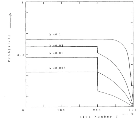
5. Numerical Experiments

We have computed the inventory distribution for some examples. In our examples the number of slots m is 300, and the reordering point r is 100, so that the reordering quantity q is 200. In this case the number of variables of the eqilibrium equations (2.2) is more than 2.0 X

logo.

On the other hand, the equilibrium equations for Pi(f2, gi) have at most 20200 unknown variables, and (4.11) which we solve indeed has only at most 100 unknown variables. We have fixed p at 1.0, and varied A from 0.1 to 0.005. When A = 0.1 for example, the mean time between placing an order and receipt of the items is ten times as long as the mean time between retrievals, i.e., when the reordered items arrive a t the system,

fm

is 90 on the average.

The results are shown in Fig. 6. As is expected, the following relations hold in the numerical results.

and the probability that each slot is full increases as the arrival rate of items A increases. We can also observe the great difference between Pr[xaoo] and Pr[x201] at A = 0.005 in particular. It means that the system often becomes almost empty by the time reordered items arrive at the system.

6. Conclusions

We consider a simple automatic warehousing system in which only one type of items are stored and retrieved, and focus our efforts on deriving the inventory distribution. This is one of the key factors in designing an automatic warehousing system. We have assumed that inventories were controlled by an ( S , S) reordering policy, and that received items are

stored from the closest open slot to the

110

point and a retrieved pallet with items is chosen randomly among currently full slots. Under further assumptions on arrival of items and request for retrieval of items the system can be modeled as a Markov chain. If we use joint inventory levels of items, the number of the states of the Markov chain amounts to 2m, where m is the total number of slots. m easily becomes several hundreds to a thousand, so that trying to solve the equilibrium equations of the Markov chain directly is not practical for real systems. So we devised exact aggregation methods for the states. The number of variables in the system of the equilibrium equations of the Markov chain has been reduced to 0 ( m 2 ) or less by the aggregation for each slot. By solving m such systems we could obtain the inventory distribution. We also developed an efficient solution method which required 0(m3) time for each system of equilibrium equations by making use of the special structure of the system. Thus the time complexity for obtaining the inventory distribution has been reduced to O(m4). This enables us to get the exact inventory distribution for real systems even though our model has simple assumptions such as only one type of items can be treated.

In order to make our model more realistic we would like to extend or apply our analysis to the following cases:

1. various types of items are treated in the system,

2. different storage methods such as class-based storage are employed,

We believe that the method presented in this paper is a good starting point to the extensions mentioned above.

Acknowledgments

The authors are grateful to the anonymous referees for their helpful comments. References

[l]

Y.

A.Bozer and J .A. White: Travel-time models for automated storage1 retrieval sys- tems.

IIE

Bansactions, 16 (1984) 329-338.

[2] D.-T.Chang, U--P.Wen, and J.T.Lin: The impact of acceleration/deceleration on travel- time models for automated storagelretrieval systems. IIE ~ansactions, 27 (1995) 108- [S] §.C.Graves W.H.Hausman, and L.B.Schwarz: Storage-retrieval interleaving in auto-

matic warehousing systems. Management Science, 23 (1977) 935-945.

[4] W.H.Hausman, L.B.Schwarz, and S.C.Graves: Optimal storage assignment in auto- matic warehousing systems. Management Science, 22 (1976) 629-638.

[5] H.Hwang and S.B.Lee: navel-time models considering the operating characteristics of the storage and retrieval machine. International Journal of Production Research, 28

90) 1779-1789.

[G] J. G-Kemeny and J.L.Sne11: Finite Markov Chains (Springer-Verlag, New York, 1976)

-

[7] A.Noguchi and S.Suzuki: An approximate solution method for obtaining the travel time

distribution of a crane in an automatic warehouse. Transactions of the Japan Society

of Mechanical Engineers, 54-C (1988) 798-804, in Japanese-

Hideaki Yamashita Faculty of Economics Tohoku University

Aoba-ku, Sendai, 980-8576, Japan. E-mail: hideakiaecon. tohoku. ac. JP