Approximate interval estimation for EPMC for improved linear discriminant rule under high dimensional frame work
35
0
0
全文
(2)
(3)
(4)
(5)
(7)
(8)
(12)
(13)
(14)
(15)
(16)
図
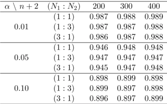
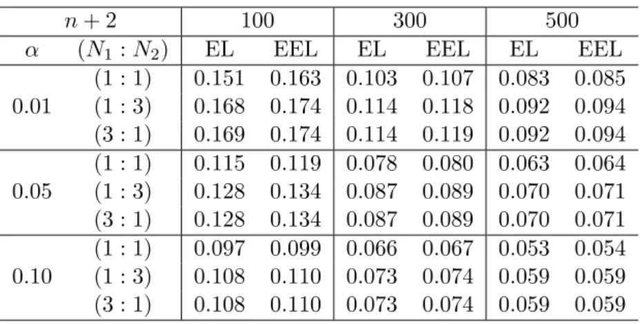

+2

関連したドキュメント
We substantially im- prove the numerical constants involved in existing statements for linear forms in two logarithms, obtained from Baker’s method or Schneider’s method
It is suggested by our method that most of the quadratic algebras for all St¨ ackel equivalence classes of 3D second order quantum superintegrable systems on conformally flat
The author, with the aid of an equivalent integral equation, proved the existence and uniqueness of the classical solution for a mixed problem with an integral condition for
In this paper we develop and analyze new local convex ap- proximation methods with explicit solutions of non-linear problems for unconstrained op- timization for large-scale systems
Our main result below gives a new upper bound that, for large n, is better than all previous bounds..
Next, we prove bounds for the dimensions of p-adic MLV-spaces in Section 3, assuming results in Section 4, and make a conjecture about a special element in the motivic Galois group
Transirico, “Second order elliptic equations in weighted Sobolev spaces on unbounded domains,” Rendiconti della Accademia Nazionale delle Scienze detta dei XL.. Memorie di
The following result about dim X r−1 when p | r is stated without proof, as it follows from the more general Lemma 4.3 in Section 4..
