Solid properties of carbon polyynes

(1)

Master Thesis

SOLID PROPERTIES OF CARBON POLYYNES

(炭素ポリインの物性)

Graduate School of Science, Tohoku University

Physics Department

MD. MAHBUBUL HAQUE

(2)

Solid Properties of Carbon Polyynes

Theoretical Condensed Matter and Statistical Physics Group Department of Physics, Graduate School of Science, Tohoku University

Md. Mahbubul Haque (A8SM2093) Background

Polyynes refer to the finite-sized molecule of lin-ear carbon chains having alternate triple and single bonds. Research on long-range carbon chains (car-byne) are being carried on since several decades. Due to the instability in air or even in solution of these linear molecules intense theoretical treatments have been carried out. It has been reported by Nishide

et al. [Chem. Phys. Letter, 428, (2006), 356-360] that polyynes are surprisingly stable inside car-bon nanotubes even at high temperature (300 ◦_C).

Once these naturally unstable molecules are found sta-ble when trapped inside single wall carbon nanotube (polyynes@SWNT) it is necessary to carry out more experimental and theoretical investigation to get in-sight of them. Tabata et al. [Carbon, 44, (2006), 3168] reported that two intense Raman shifts appear around 2000 -2200 cm−1_{. Regarding the intensities}

of these two bands these are categorized as α-bands (most intense bands) and β-bands (2nd most intense bands). The nature of these two bands is to decrease in frequency with the increase in polyyne size. The de-creasing nature of α-bands is almost linear with chain lengths whereas that of β-bands is oscillating that is the difference in frequency shifts between β-bands and α-bands are not similar in all polyyne molecules. Malard et al. [Phys. Rev. B, 76, (2007), 233412] reported in his resonance Raman spectroscopy exper-iment of C10H2@SWNT and C12H2@SWNT that the

strongest Raman intensity due to polyynic “P” bands observed for laser excitation around 2.1 eV. In order to analyze Raman features it is necessary to examine vi-brational frequencies of possible Raman active modes and also to examine of excited states energies. Nuclear magnetic resonance (NMR) experiment reported by Wakabayashi et al. [Chem. Phys. Lett., 433, (2007), 296]. They noticed that the chemical shifts of13_C

nu-clei decrease at a cooling temperature of -10◦_{C whose}

analysis is requested.

Purposes

The purpose of this thesis is to analyze Raman fea-tures of polyynes and hence to calculate the frequen-cies of normal modes of vibration. We calculate ex-cited states energies of bare polyynes in order to com-pare Raman excitation profile of polyynic P bands of polyynes@SWNT hybrid systems. We also perform NMR calculation of polyyne molecules in order to get the features of nuclear spin-spin coupling constants as a function of distance between the spin-1/2 nuclei (i.e.

1_{H and}13_C).

Calculation methods

Figure 1: Shows calculated results vibrational frequen-cies of Raman active mode (triangle-down) of a series of polyynes C2nH2; n=4-8, which are comparable with

the experimental Raman shift α-bands (triangle-up) [Tabata et al., Carbon, 44, (2006), 3168]. The cal-culated results are obtained by DFT (B3LYP) with 6-311G(df,p) basis set and the results are scaled by scaling factor 0.961.

Figure 2: Shows calculated results for vibrational fre-quencies of Raman active mode (open-circle). Other explanations is similar to that of Fig. 1

We use Gaussian09 software package as our calculation tool. Both Hartree-Fock and density functional the-ory (DFT) methods are used for geometry optimiza-tion and vibraoptimiza-tional frequency calculaoptimiza-tion. In DFT we use Becke-3 parameters-Lee-Yang-Parr (B3LYP) func-tional. In the case of excited states calculation the molecular geometries are optimized by DFT (B3LYP) functional and energies are calculated by CIS (con-figuration interaction with single excitation) method. For NMR (nuclear magnetic resonance) calculation optimized structures are obtained by DFT (B3LYP) along with 6-311G+(2d,p) basis set and NMR calcu-lation carried out by gauge independent atomic orbital

(3)

Figure 3: Shows singlet excited states energies of a series of polyynes at the different optimized structures. The calculation is performed using CIS method. (GIAO) method. Chemical shift is obtained as relative shifts from that of TMS (tetramethylsilane).

Results and Discussion

(1)Vibrational properties: In our calculation of vi-brational frequencies for C8H2 to C16H2 we find the

frequencies of two possible Raman active modes hav-ing highest scatterhav-ing activities lie between 2000-2200 cm−1 _{which are in good agreement with the}

experi-mental Raman shifts of α− and β−bands. Also we find that between the two Raman active modes the higher frequency mode, α−mode, decreases linearly with increasing lengths of polyyne molecules and the lower mode, β−mode, decreasing with polyyne lengths but possesses oscillating behavior. These two modes of vibration may be responsible for the experimen-tal Raman shifts of α− and β−bands. Figs. 1 and 2 show the calculated of vibrational frequencies which are compared with the experimental data [Tabata et

al., Carbon, 44, (2006), 3168]. The calculated results

are scaled with a scaling factor 0.961.

(2) Excited states energies: Fig. 3 shows the calcu-lation results for excited states energies of polyynes, H − (C ≡ C)2n− H; n= 4-8. We see that the

exci-tation energies decrease with the increase of polyyne size. We predict energies of first three lowest excited states using different basis sets.

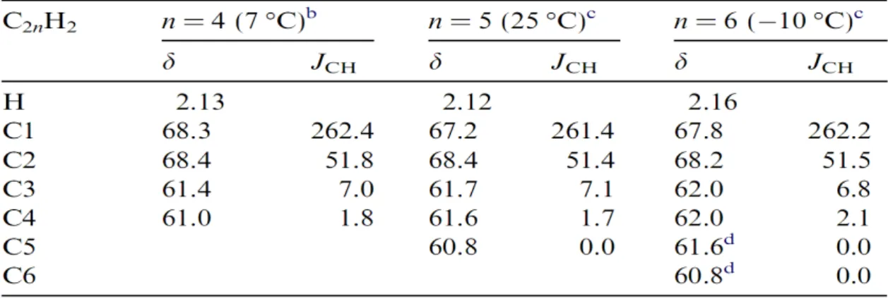
(3) NMR calculation: Table 1 shows the calculated results for chemical shifts of 1_{H and} 13_{C nuclei at}

different polyyne molecules which are compared with experimental results [Wakabayashi et al., Chemical Physics Letters, 433, (2007), 296]. The first column represents the position of 13_{C nuclei referenced from}

the1_{H nucleus at the one end. We see the calculated}

results for chemical shifts are in good agreement with experimental results.

In Table 2, we see that the coupling constant JCH

due to spin-spin coupling between 1_{H and} 13_{C nuclei}

varies with the distance between them. We see that the values of JCH, for the identically positioned 13C

nuclei, also vary with the molecular size. For instance, in molecule C8H2 the coupling constant between 1H

Table 1: Calculated data for chemical shifts, δ, (ppm) of1_{H and}13_{C nuclei in different polyyne molecules.}

Table 2: Calculated results for spin-spin coupling con-stants in Hz (JCH) between1H and13C nuclei in which

the positions of13_{C nuclei are referenced from}1_H

nu-cleus.

and 13_{C, in which} 13_{C at the position of first nearest}

neighbor (i.e. C1) to 1_{H, is 262.4 Hz (experimental)}

and 254.8 Hz (calculated) which is different from the coupling constant for the similarly positioned 1_{H and} 13_{C nuclei in C}

10H2is 261.4 (experimental) and 255.4

Hz (calculated) respectively. We observe similar be-havior in the case of coupling constant JCC due to

coupling between13_{C nuclei.}

Conclusion

Our calculated results for Raman active modes (α− and β−modes) can be attributed to the experimen-tal Raman shifts (α− and β−bands). We find DFT(B3LYP) along with 6-311G(df,p) basis set can produce experimental results more closely. We can give some explanations for the frequency decreasing nature of α− and β−modes. Calculated results of NMR give good agreement to experimental results of chemical shifts and spin-spin coupling constants.

Presentation

“Vibrational spectra and excited states calculation of polyynes@SWNT”, M. M. Haque, R. Saito, 38th Fullerene-Nanotube symposium, Meijo University, Nagoya, March 2-4, (2010).

(4)

Acknowledgments

I would like to express my deepest gratitude to Professor Riichiro Saito for his guidance during my Master course study. I would like to express my hearty thanks to Dr. W. Izumida, Dr. Jin Sung Park and Dr. Li-Chang Yin for their encouragement and friendly discussion related to academic as well as daily life matter. It is also my pleasure to express my hearty thanks to my friends R. Endo, M. Tareque Chowdhury, A.R.T. Nugraha and M. Furukawa, T. Eguchi, Yutaka Oya and Daisuke Yabe for their fruitful discussion on physics and who made many funny activities which are good sources of mental recreation. I must acknowledge MEXT for Monbukagakusho scholarship support that makes it possible to pursue my studies in Tohoku University.

(5)

(6)

Chapter 1 Introduction

1.1 Purpose of this study

Polyynes are the general name of such a class of molecules having alternate single and triple bonds and hence the general formula of such liner carbon chains can be written as -(C ≡ C)n-, where n is an integer, (n = 2, 3, ...up to a finite even value. For n = ∞ it is called carbyne). Thus polyynes are finite sized perfect sp-hybridized molecules. The terminals of the molecules can be terminated by atoms or group of atoms. Hydrogen terminated polyynes H(C ≡ C)nH are the simplest form of polyynes. Both the experiment and theory have revealed the bond structure of polyynes; for instance, Longuet-Higgins and Burkitt [1] and Hoffman [2] have shown that polyynes are chemically bonded with alternatively single and triple bonds. Cyanopolyynes, H(C ≡ C)nC ≡ N, where (n= 1.... 5), a member of polyyne group was detected in the interstellar space by radio astronomy in 1970s [3–6]. The basic properties of polyynes are; these are unstable in air even in liquid at high concentration [7].

The purpose of this thesis is to calculate some solid properties of polyynes including their vibrational frequencies, nuclear magnetic properties and excited states energies. The intention of some of these calculations is to reproduce some experimental results and to have some clear explanations. For example, in order to analyze the Raman spectroscopy experiment for polyynes it is important to

(9)

2 CHAPTER 1. INTRODUCTION calculate normal mode of vibrational frequencies of polyynes giving emphasis on the possible Raman active modes.

As a motivation of this work it can be mentioned that it is necessary to examine properties of polyynes in more detail. Polyynes are expected to be better candidates for doping agent than the carbon nanowires (CNWs) because polyynes are smaller in size than CNWs and as Xhao et al.(2003) reported that a long chain of CNWs was found to be stable inside the inner most CNT of multiwall carbon nanotubes, it is natural to expect polyynes to be more stable inside single wall carbon nanotubes (SWNTs). It is clear that the stabilization of doping agent inside the host material is an important factor. Once the doping material is stable inside the host, we can examine the various properties of the hybrid system through both theoretical and experimental ways. It is quite natural to start our theoretical treatment of simply polyynes because the calculation for the hybrid system would seem to be difficult. In the case of NMR results reported by T. Wakabayashi et al. (2007), the reason of dependence of chemical shift on temperature is not explained in their paper. So a comparative study through NMR calculation of polyynes is also needed. In future we will extend our calculation for the hybrid system i.e. polyynes inside SWNTs (polyynes@SWNTs).

Polyyne compounds are also available in nature with varieties of structural diversities and features. Ferdinand Bohlmann, in his book Naturally occurring

acetylenes, reported that “dehydromatricaria easter”, the first natural acetylene,

found in “Artemisia” species in 1986. Up to present more than thousands of polyyne compounds have been found in nature e.g. in fungi, bacteria, marine sponges and corals etc. [8–13]. G.H.N. Towers (1978, 1984, 1997) and J.B. Hud-son (1993) in their works and in other several articles [14–17] it has been re-ported that such compounds posses their unique properties that are useful for varieties of biological application such as antibacterial, anti-microbial, antifungial, anti-tumor,anticancer, anti HIV (human immunodeficiency virus) and pesticidal

(10)

1.2. BACKGROUND 3 properties . As polyynes are almost perfect in linear and hence their conjugate π electrons are doubly degenerated they are expected to be a candidate for molecular devices as well as molecular wires [18] Polyynes are found unstable in air(solid phase) even in liquids (diluted phase) at high concentration [7]. Due to their in-stability theoretical treatments have been carried out intensively in order to reveal their electronic properties and other several physical properties [19–22]. These often unstable molecules are surprisingly stable inside carbon nanotubes [23] even after several months the polyynes are stable inside SWNTs. Encapsulation of polyynes of different lengths inside SWNTs also have been confirmed by the Ra-man spectroscopy method of polyynes@SWNT [24].

1.1.1 Organization

We will arrange our thesis as follows: we discuss about the background of our work in this chapter. As a background we briefly discuss about some experimental works including synthesis and detection process of polyynes, Raman experiment of polyynes, Raman experiment of polyynes@SWNTs as well as experimental results on Raman excitation profile of polyynes@SWNTs. We also include to the NMR experimental results of polyynes. The chapter 2 is furnished by describing the calculation methods that used in our calculation. In chapter 3 we will include the calculated results of normal modes of vibration and in chapter 4 we will include excited states energy results and NMR results. Summary will be presented in chapter 5. We also include an appendix at the end of this thesis.

1.2 Background

In order to describe the background of this work it is necessary to mention here some basic information about the synthesis, detection as well as characterization process of polyynes. In order to explain our motivation to this work we will

(11)

intro-4 CHAPTER 1. INTRODUCTION duce some experimental results those have been obtained for both polyynes and polyynes@SWNTs. Why we will introduce the experimental data of polyynes@SWNTs because our main intention, in future, to extend our calculation for that hybrid sys-tems.

1.2.1 Synthesis and detection of polyynes

The synthesis of polyynes in liquid phase was achieved in 1972 through the clas-sic synthetic approach of organic chemistry involving the Cu-catalysed oxidative couplings, so called Hay technique, of silyl-protected terminal alkynes [25]. Laser ablation method, currently, is one of most popular methods for the synthesis of carbon clusters including C60, carbon nanotube, carbon nano-wire etc. Polyynes, a form of carbon cluster, can be achieved by the laser ablation of graphite. This method can be taken place in both the gas and liquid phases. Even though the gas phase of this method has been studied for a long time after the discovery of C60, recent trend is to the liquid phase. In the case of liquid phase the liquids which are used as the suspension of graphite particles, usually, are toluene, benzene, n-hexane etc. [26]. The laser beams that are used to irradiate the graphite sample are of about 530 nm. The irradiation process takes several hours. As graphite particles are soluble into such liquids, the insoluble parts are removed filtration process. This soluble parts (solution) may consists of different types of carbon clusters including polyynes of different lengths. In order to get the desired product the solution of each of those products is separated by Hi performance Liquid chro-matography (HPLC) technique. Finally the separated solutions are subjected to some spectroscopic analysis. The Figs. 1-1(a) and (b) are the schematics of typical laser ablation method as well as of HPLC respectively. In Fig. 1-1(b) the spots in the array of vertical direction at different retention time i.e. at 5.3, 6.3, 9.1, and 16.4 minutes refer to the absorption of UV (ultra violet) wavelengths by C8H2, C10H2, C12H2, C14H2 respectively.

(12)

1.2. BACKGROUND 5

(a) (b)

Figure 1-1: (a) shows schematics of laser ablation cell of graphite particles sus-pended in solution [26] and (b) shows two dimensional High Performance Liquid Chromatography (HPLC) on the separation of several polyyne molecules. The contours represent UV absorption intensity corresponding to the detection wave-lengths as a function of retention time [24].

In order to detect as well as to characterise the polyynes most experimental researchers use the ultra-violet/visible (UV/Vis) spectroscopy. UV/Vis method, which deals with electronic transitions, is a good tool for quantitative analysis of molecules. In 1972, Eastmond et al. has successfully synthesis a series of polyynes (up to n = 4....10, 12). His UV/Vis spectra for those polyynes are still being used as a reference or standard one to recent researchers. The Fig.1-2 is the typical UV/Vis spectra of different length of polyynes recently synthesized using laser ablation of graphite particle method in liquid phase [27].

In Fig.1-2 it is shown that the absorption wavelength increases with increasing size of polyyne molecules. This absorption UV spectra is the characteristic features to identify the polyynes in n-hexane solution. The small speaks pointed by down arrows are due to the impurities.

Fig. 1-1: figure/laser-ablation.eps, figure/hplc.eps Fig. 1-2: figure/UV-spectra.eps

(13)

6 CHAPTER 1. INTRODUCTION

Figure 1-2: Typical UV/Vis spectra of a series of polyynes [27].

1.2.2 Raman experiments on polyynes

The Figs. 1-3 represent typical normal Raman spectra of a series of polyynes ob-tained by Tabata et al. [27]. In their experiment the polyynes were prepared by using laser ablation method of graphite particles in n-hexane and similar method as mentioned in the previous sub-section. For the Raman experiment purpose each of the separated solutions contain different size of polyyne has been irradiated by Ar+_{laser of 532 nm line.}

(14)

1.2. BACKGROUND 7

(i) (ii)

Figure 1-3: (i) Raman spectrum of solution of n-hexane and C8H2(upper solid line) and Raman spectrum of pure n-hexane (bottom dashed line). (ii) Net Raman spectrum of C8H2obtained by subtracting between the two spectrum of (a) Raman spectra of a series of polyynes C2nH2; n = 4...8. A DFT calculation results for Raman active modes are shown by vertical bar A and B [27].

Fig. 1-3(i) shows the procedures of extracting net Raman spectra of polyyne molecules suspended in liquids (n-hexane). Due to the presence of n-hexane a background spectra appears along with the polyyne spectra, which is shown by the bottom spectra of Fig. 1-3(i:a) and the upper spectra represents the Raman spectra of C8H2 in n-hexane. The Fig. 1-3(i:b) shows the net Raman spectra for polyyne ( C8H2) which is obtained by subtracting the spectra due to n-hexane from the Raman spectra of polyyne in hexane. Following the similar way the net Raman spectra of other longer polyyne chains i.e. of C10H2, C12H2, C14H2, C16H2

(15)

8 CHAPTER 1. INTRODUCTION is obtained which is shown in Fig. 1-3(ii). We can see from the Fig. 1-3(ii:a-e) that between the two prominent peaks of each molecule the highest intense band is denoted by α-bands and the second highest intense band is attributed as β-bands. It is clear to see that both the α- and β-bands red shifted with the molecular size of polyynes. The shifting nature of α-bands is almost linear but that of β−bands is not linear that is the shifting varies with molecular size. In addition to the oscillation shifting nature of β-bands it also appear at higher frequency region for C16H2. The vertical bars A and B represent the Raman scattering activities of vibrational frequency obtained by density functional theory (DFT) calculation for vibrational frequency of polyynes using Becke-3-parameter-Lee-Yang-Parr (B3LYP) functional with correlation consistent polarized valence double-zeta (cc-pVDZ) basis set. On the basis of the Raman scattering activities and corresponding frequency values these two vertical bars A and B seem to be relevant to place in the Raman shift positions of Raman spectra.

1.2.3 Raman experiments on SWNTs

Here, in brief, we need to introduce the synthesis process of carbon nanotubes because it is necessary to have this knowledge in order to understand the synthesis process of polyynes@SWNTs, which we will discuss in the next section. There are several methods of SWNT synthesis, such as; arc discharge [28], laser ablation [29], chemical vapor deposition (CVD) [30] etc.. Here we will confine ourselves to discuss about laser ablation process only. Although this process is almost similar to that of polyynes but in the case of carbon nanotubes the synthesis process is carried out at high temperature (around 13000_{C). The metal that contains carbon} is put into a quartz tube. The Ar gas is passed through the tube. The Ar gas flow is then heated with high temperature at 12500_{C [23] with the help of a furnace. The} quartz tube that act as a target is then irradiated for several hours (e.g. 3 hours) by a laser source (for example Nd:YAG) whose laser lined is maintained at around 530

(16)

1.2. BACKGROUND 9

Figure 1-4: Typical Raman spectra of SWNTs [31]

nm. The irradiation are of the target and the area of the laser beam are of the order of millimeter. The obtained soot-like mixture, through this process, may contain fullerenes and other carbon clusters in addition to carbon nanotubes. To make the carbon nanotubes free from impurities for instance; from fullerenes usually toluene is used because fullerene is a good solvent of toluene. Hydrogen per-oxide and hydrogen chloride together is used to remove metallic and other impurities. In this stage a film-like product of carbon is achieved that contains mostly carbon nanotubes. This film is then dried by heating it at about 500 0_{C. Finally the} Raman spectroscopy is used to characterize the nanotubes. The following Fig. 1-4 represents typical Raman spectra for both metallic and semiconducting SWNTs [31]. From the Fig. 1-4 we can see several peaks, in which the peaks at the lower frequency region are called radial breathing mode (RBM) due to the vibration of carbon atoms in the radial direction [31]. RBM mode is very sensitive to nanotube diameter and its values range from 120-350 cm−1 _{within the diameter range of}

(17)

10 CHAPTER 1. INTRODUCTION 0.7 nm to 2.0 nm [31]. The nomenclatures of other bands i.e. D, G, G’ were established in the field of graphite but they are still familiar with the same name in the carbon nanotube field with different values. The peak so-called “D-band” is appeared at around 1350 cm−1_{which is due to the Raman scattering in disordered} graphite [32]. The band denoted by G’ arises near around at 2700 cm−1 _{that is this} position is almost double to that of D band. Actually both the D and G’ bands are the double resonance processes. For our purpose we will not discuss details about all other peaks i.e. M, iTOLA etc. We will concentrate to the Raman spectra of polyynes@SWNT in order to understand the encapsulation of polyynes inside SWNT.

1.2.4 Raman experiments on polyynes@SWNT

Before showing the Raman experiments of polyynes@SWNT, we would like to mention , in brief, the procedures of trapping polyynes inside SWNT. Experimen-tally, there could be several ways to mix the polyynes with SWNTs in order to encapsulate polyynes into SWNTs, here we will mention the method followed by Nishide et al. [24]. The encapsulation process of polyynes into SWNT are carried out by pouring polyynes solution at the one end of a Y-shaped glass ampoule and the film SWNTs at the other end of the ampoule. The n-hexane solution of polyyne is kept frozen with the help of liquid nitrogen and the film of SWNTs are kept warm by heating at low temperature with the help of a Bunsen burner. Finally both ends of the ampoule kept sealed for about 2 days keeping the system at a temperature about 80 0_{C. To make sure that the polyynes are really trapped by SWNT Raman} spectra for the hybrid system is analyzed. The following is the typical Raman spectra of the hybrid system containing polyynes and SWNTs.

In Fig. 1-5 we can see that the RBM, D, G and G’ bands, typical bands that usually appear in the case of SWNTs, are common for both the spectra of pristine nanotube

(18)

1.2. BACKGROUND 11

(a) (b)

Figure 1-5: (a) Shows Raman spectra of C10H2@SWNT. At the bottom (black line) the spectra is obtained for the pristine SWNT and on the top (red line) the spectra obtained for the hybrid system. (d) Shows the similar Raman spectra in which the bottom (black line) one representing Raman spectra of pristine SWNT while on the top it represents Raman spectra of C2nH2@SWNT (n = 4 . . . 6) (red line) [24].

(black line) and of hybrid system i.e. polyynes plus nanotube. It can be seen easily that an additional band is appeared around 2066 cm−1 _{for the hybrid system (red} line). The additional band is to be expected due to the existence of polyynes in that hybrid system this peak position is comparable with that of the Fig.1-3 which is the Raman shift for C10H2having the value of 2123 cm−1. This numerical deviation by 57 cm−1_{in peak position could be due to the interaction between the trapped C}

10H2 and the SWNT. Nevertheless, the nature of the bands in both cases are sufficiently similar to think of C10H2 be encapsulated inside SWNT. In order to confirm the encapsulation of C10H2 in more evidently the X-ray powdered diffraction (XRD) spectroscopy for both the hybrid system as well as for pristine SWNT have also been obtained, which is shown in the Fig.1-6. The figure shows that in the case of the hybrid system the peak intensity at 0.4 Å−1_{falls with great value (red line)} in comparison with that of the pristine SWNT (black line). This type of behavior

(19)

12 CHAPTER 1. INTRODUCTION

Figure 1-6: XRD-spectra of C10H2@SWNT (red line) and that of pristine SWNT is (black line)

is considered as a proof of encapsulation of objects inside SWNTs that has been reported in [33–35].

Figure 1-7: Shows Raman intensity of polyynic, P, bands for C10H2@SWNT (up-per closed triangles) and C12H2@SWNT (lower open circles). Figures show that intensities are maximum at around 2.1 eV laser excitation energy

Malardet al. carried out Resonant Raman spectroscopy experiment of C10H2@SWNT and C12H2@SWNT [36]. In his experiment several different laser lines are used to get strong Raman signal due to polyynic, ’P’, bands. Fig. 1-7 shows the Raman excitation profile of P-bands when polyyne molecules encapsulated inside SWNT.

Fig. 1-6: figure/x-ray-pol-at-cnt.eps

(20)

1.2. BACKGROUND 13

Table 1.1: Experimental data on chemical shift δ and spin-spin coupling constants (ppm) JCHbetween1H and13C nuclei.

From this figure it is seen that the higher resonance intensities of P bands occur at laser energies range from 2.0 to 2.3 eV. In the case of C10H2@SWNT the maximum intensity occurs at 2.14 eV and that of C12H2@SWNT occurs at 2.10 eV. In our cal-culation for excited states energies of polyynes in Chapter 4 we will compare this experimental results with our calculated results.

1.2.5 NMR experiments of polyynes

T. Wakabayashi et al. performed nuclear magnetic resonance (NMR) experiment on C8H2, C10H2and C12H2molecules in n-hexane ??. The following table 1.1 shows the data for chemical shift δ (ppm) of13_{C and}1_{H and spin-spin coupling, J}

CH (Hz), between13_{C and}1_{H at different temperature. It can be seen clearly that the chemical} shifts data for carbon nuclei are changing with temperature.

In the Table: 1.1 the first column (from the left) holds for the isotopic positions of1_{H and}13_{C isotopes relative to each other. The atomic label C1 of the C nucleus} refers to the first nearest neighbor 13_{C atom to} 1_{H atom in the hydrogen-caped} polyynes. Similarly the C2, C3, C4 and so on refer to the second, third, fourth and so on nearest neighbor of 1_{H nucleus respectively. The purpose of placing}

(21)

14 CHAPTER 1. INTRODUCTION 13_{C atoms at different position relative to}1_{H atom is clear, that, they measure the} values of coupling constants JCHas and chemical shift δ as a function of the distance between H and C isotopes. The 2nd and 3rd column is for the chemical shift, δ and coupling constant values for C8H2 molecule at a temperature of 70C. The 4th and 5th columns are presenting similar data for C10H2 molecule at temperature of 25 0_{C while the column seven and eight are presenting the same for molecule C}

10H2 at temperature -100_{C. It is clear to observe that the chemical shift is changing at a} cooling temperature -100_C.

(22)

Chapter 2 Calculation Method

2.1 Introduction

All most all of our calculated results are obtained by first principle calculation. We used both Hartree-Fock (HF) and density functional (DFT) approach. The reason of using both of those methods is, mainly, to compare the result quantitatively. Also we have compared the calculation cost for these HF and DFT methods. Even though, it is well known that the DFT calculation is less expensive in comparison with HF method, nevertheless, we like to understand exactly how these methods differ each other in our case. Gaussian software package i.e. “Gaussian 09” and “Gauss View 5” have been used as the calculation tools in most of our calculations. Gaussian and Gauss View are two separate software packages. Main calculation is done by Gaussian package while GaussView is a very helpful tool to make the calculation environment more friendly. Hence we can run Gaussian calculation, usually, in two ways: one is to configure input file of calculation directly on the input panel of Gaussian software interface, and another way is to configure input file with the help of Gauss View package. In order to run program directly on Gaussian package we need to declare job type, atomic or molecular specifications such as atomic number, atomic coordinates, boding types, etc. manually. Usually

(23)

16 CHAPTER 2. CALCULATION METHOD

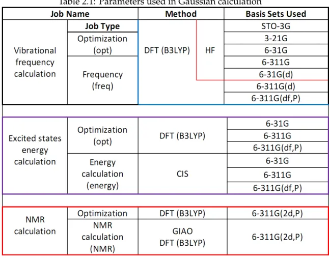
Table 2.1: Parameters used in Gaussian calculation

the use of Gaussian package is little bit unfriendly and time consuming. On the other hand one can do the above operations with the help of GaussView easily within very short time. Hence the role of GaussView is not only to help to build the molecular structure and to configure the input files but also help to analyze as well as visualize the output of calculations. In our calculation we use GaussView to run the Gaussian calculation because it is possible to run the Gaussian program from the GaussView interface. Once Gaussian package in installed on a computer the further installation of GaussView creates a link with the Gaussian software automatically. The Table 2.1 shows, at a glance, the parameters used for our calculation.

In Appendix we include the procedures of using GaussView in more system-atically. However, in the following sections of this chapter we will show, mainly,

(24)

2.1. INTRODUCTION 17 how to set the above parameters of Table 2.1 for different jobs with the help of GaussView. In brief, the first column (“Job Name”) represents the main calculation types, i.e. calculation for vibrational frequencies, excited states energies and NMR calculation. Each calculation is divided into two sub-calculations which must be carried out to get the more accurate calculation results. For example, each main calculation consists of the calculation for geometry optimization. Optimized ge-ometry is itself not a abstract matter, that is, better optimized structure depends on the use of calculation methods as well as on the choice of basis sets. It is usu-ally expected that larger basis sets result more accurate optimized structures. In the Table 2.1 the 2nd column (“Method”) represents the calculation methods used in our calculations. For vibrational frequency calculation both the Hartree-Fock (HF) and density functional theory (DFT) with Becke-3 parameter-Lee-Yang-Parr (B3LYP) functional are used. For excited states energy calculation the configura-tion interacconfigura-tion (CI) method is used. CI method is a common terminology, in our calculation, the CI method is based on such wave function which is expressed as a linear combination of all determinants formed by replacing a single occupied orbital with a virtual orbital hence this method is termed as CIS [37]. The NMR cal-culation is performed by gauge independent atomic orbital (GIAO) method. The 4th column represents a list of predefined basis sets that are used in our calculation. It is noticed that for the same calculation we use different sets of basis sets in order to get more accurate results as well as to compare the results both qualitatively and quantitatively. The meaning of the symbolic representation of the basis sets are well known.

(25)

2.2 Running Gaussian programs

2.2.1 Building polyynes structure and optimization of geometry

After running GaussView it is easy to build polyyne structures by adding even number of several carbon-divalent (single-triple) unit structures in a linear fashion. (in appendix we shown how to build polyyne structure). Polyynes, built in this way, are not geometrically optimized that is the initial bond lengths, bond angles obtained by this way should not be used for molecular calculation. The first and principle condition of any electronic structure calculation is to obtain optimized geometry of the sample. Geometry optimization refers to the finding of the total energy of the system as minimum as possible and the corresponding bond lengths, bond angles, dihedral etc.. The optimized geometry is not an abstract matter rather it depends on the methods of calculation, basis sets etc.. In the Table 2.1 we men-tion that for vibramen-tional frequency calculamen-tion purpose we optimize the polyyne geometry by using both HF and DFT (B3LYP) along with different Gaussian basis sets starting from smallest basis set i.e. STO-3G up to comparatively larger basis set 6-311G(df,p).

The Fig.2-1 shows the available several calculation options provided by the Gaussian package. On this interface there are several “tabs” which are providing different several existing calculation options. The left most tab “Job Type” provides the main calculation option. We can select only one job type at a time except for frequency calculation we can set two jobs at the same time, that is, with the selection of “Opt+Freq” option we can run program for both optimization and frequency calculation. The program will run for for obtaining optimized structure and after that it will calculate vibrational frequency. In most of our calculation for vibrational frequency we use this option. The “Method” tab provides to set either ground state calculation or excited state calculation. Vibrational frequency calculation requires to set ground state calculation. For the calculation method HF is set by default.

(26)

2.2. RUNNING GAUSSIAN PROGRAMS 19 Once DFT method is set then additional field is appeared to select DFT functional. By default the B3LYP functional is set for DFT calculation. The spin state of the system is set as “Default Spin” by default. This option is same as to select the “Restricted” option. Either of these option refers to such system (molecule) in which there are no unpaired electrons. In all of our calculations we select “Default Spin” option. In the case of DFT calculation we use B3LYP functional. This is a hybrid functional, which stands for Becke-Lee-Yang-Parr (BLYP) functional. The numerical integer “3” comes with this functional as there are three empirical parameters used in the pure BLYP functional. The reason of selecting this hybrid functional is straight forward that is, currently, it is the most popular functional because the three empirical parameters used here in such a way that this functional can reproduce some atomization and ionization energies as well as some total energies in such optimal way that can be compared with the G2 (Gaussian-2) database [38]. It is well known that G2 database is based on well-established Gaussian-2 theory in which the theory is able to reproduce experimental data with higher accuracy. There are several predefined basis sets are available to select it from the basis sets list. In most of our calculation we repeat the same calculation only changing basis sets.

(27)

Figure 2-1: shows the available several calculation options provided the Gaussian package and how those options can be used by GaussView. From the left, under the “Job Type” tab we can assign job for optimization, frequency, optimization plus frequency together with single command “opt+freq”, other calculation options including NMR calculation. Under the “Method” tab we can set molecular state, for instance; ground state, basis sets, calculation methods i.e. DFT, HF MP2 etc.. It can be noticed that once DFT method is set another tab (right most one) will appear to select the DFT functional e.g. LSDA, B3LYP etc. The second right most option is to set the system as closed shell restricted/unrestricted or open shell unrestricted. By default it is set as “Default Spin” which is same as to select “Restricted” option

(28)

2.2. RUNNING GAUSSIAN PROGRAMS 21 For the optimization purpose we run our calculation by both HF and DFT meth-ods. We used similar basis sets for both methmeth-ods. The default memory is ,although, 48 MB is allocated, but in order to avoid unexpected termination of program due to lack of memory, we increase memory size to 1 GB in most of our cases. This option i.e. assignment of memory can be carried out under the tab “Link 0” of Fig.2-1. It has been found that for the small sized polyynes C2nH2; n = 4 − 6 we had normal termination of program but for the larger polyynes i.e n= 7-8, the program termi-nated abnormally due to inability to reach the convergent state. That is the default number for SCF cycles were not sufficient to achieve the convergence of energy, force and displacement etc.. In these cases we use forced convergence method. The use of forced convergence method is comparatively expensive than ordinary SCF calculation because in the later case the the number of SCF cycles are such a large that there is a guarantee to reach a stationary point. And hence the com-putation cost increases. After successful completion of optimization calculation we open the Gaussian output file whose file extension is“.log”. We check the four basic entities, namely, maximum force, RMS (root mean square) force, maximum displacements and RMS displacements, which are converged. The convergence criteria are defined by some threshold values. We use the default threshold values for the above four entities. We also check that the optimized orientation of the polyynes molecules are exactly alone z-direction, since polyynes are one dimen-sional linear structure, while the input orientation (before optimization) is along xyz-plane. Also the optimized bond angle is exactly 180◦ _{between two atoms. In} order to understand the optimized structure we also check the derivatives potential energy with respect to distance reach to zero which is the condition of energy to be minimum. From this output file we also get the data for total time that is used to complete the calculation. Finally we achieved optimized structures for all of our polyyne molecules. The optimized data are included ,in tabulated form, at the appendix section of this thesis.

(29)

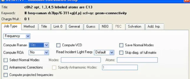
Figure 2-2: shows the frequency calculation procedure and setting up the parameter to calculate Raman active mode. The field “Compute Raman” should be set to “Yes” in order to instruct program to calculate possible Raman active modes of vibration. By default the Gaussian program does not calculate Raman activities.

2.2.2 Calculation of normal mode of vibration

Calculation for normal modes of vibration is carried out together with the opti-mization calculation, as mentioned above, by setting the keyword “opt+freq”. In order to calculate the possible Raman active modes of vibration we select the “com-pute Raman =Yes” as shown in Fig.2-2. By default the program does not calculate Raman active modes but infrared (IR) active modes of vibration.

2.2.3 Calculation of excited states energies

Configuration interaction (CI) method is used to calculate singlet excited states energies. Under the method tab, except “ground state” option, all the keywords i.e. ZINDO, CIS, SAC-CIS, TD-SCF and EOM-CCSD are used to perform excited states energy calculation. In our calculation we used the keyword CIS (CI-Singles). CIS is a model of configuration interaction approach in which excited states are treated

(30)

2.2. RUNNING GAUSSIAN PROGRAMS 23

Figure 2-3: shows the excited state energy calculation settings. The CIS keyword instruct the program to calculate excited states energies with configuration inter-action method. The default value of “Root” section is 1 which indicates that by default it will calculate the first lowest excited states.

as the combinations of single substitutions of HF wave function. As mentioned above, in this method an occupied spin orbital is substituted with a virtual spin orbital. The geometry optimization calculation for this purpose is also carried our at excited states instead of ground state because it is recommended that in order to calculate excited states energy the geometry of the system should be optimized in that excited state also. Using only three basis sets namely 31G, 311G and 6-311G(df,p) we performed our calculation and compared the results to understand the basis sets dependence of energy. It is necessary to specify which excited state is to be studied for both optimization and energy calculation. We did not set this option because our intention is to calculate first (lowest) excited state energies and by default Gaussian calculates first three lowest excited states. The Fig.2-3 illustrates the input file settings for excited state energy calculation.

(31)

2.2.4 NMR shielding tensors and chemical shift calculation of

polyynes

In order to calculate NMR it is a must to configure atoms or molecule with desired net non-zero spin. In our purpose of NMR calculation for spin-1

2 system we replace the 12_{C atom with} 13_{C isotope while we change H nuclei because by default} 1_H nuclei is set. Gradually we replace all 12_{C atoms within the center of symmetry} of polyyne molecules with 13_{C isotopes in order to calculate spin-spin coupling} constants (JCH) and (JCC) between 1H - 13C and 13C- 13C respectively as a function of distance between these spins. The Fig.2-4 shows how to edit atomic list to set spin isotopes. Clicking the icon “bold A”, invokes “Atom List Editor” panel. We can see that there is a option to change the atomic mass number. For example, the default mass number of C atom is set as 12. In order to perform NMR calculation we set mass number for C atom as 13.

Geometry optimization is done by DFT(B3LYP) method along with 6-311G+(2d,p) basis set because this method and basis set is also used to calculate NMR of TMS (tetramethylsilane) and Gaussian used the result of TMS calculation as a reference to calculate chemical shift of1_{H or}13_{C in other molecules. In order to perform NMR} calculation in the job type section we set “Job Type =NMR” along with the keyword “GIAO method” the stands for “gauge independent atomic orbital method” which is one of the most popular method for NMR calculation. Besides we set, under the “Method” tab set DFT(B3LYP) as calculation method with 6-311G+(2d,p) basis set because the same basis set is used to optimize polyynes structure.

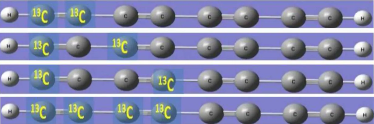
In Fig. 2-5 we illustrate how to build i.e. configure molecular structure by placing13_{C nuclei at different locations in order to calculate the spin-spin coupling} constants JCH between 1H and13C nuclei as a function of distance between them. Here we show the process only for C8H2 molecule and similar procedure can be applied for longer molecule and due to the symmetry only we need to do this up

(32)

2.2. RUNNING GAUSSIAN PROGRAMS 25

Figure 2-4: Shows the option to edit the atomic list in order to set the mass numbers of atoms. For NMR calculation the mass number of C atom should be changed from default value 12 to 13

to the center of symmetry.

Fig. 2-6 shows examples of increasing13_{C nuclei in polyyne molecules in order} to calculate spin-spin coupling constants (JCC) between 13C and 13C nuclei as a function of distance between13_{C nuclei. We repeat this process for polyyne C}

2nH2 molecules up to n=4 . . . 8. Of course, with this configuration it is also possible to calculate the coupling constants (JCH) at the same time.

Fig. 2-5: figure/H-C-coupling-configuration.eps Fig. 2-6: figure/JCC-JCH-all.eps

(33)

Figure 2-5: Shows how to arrange 13_{C nuclei in polyyne molecules in order to} calculate spin-spin coupling constant (JCH) between1H and13C nuclei as a function of distance between them. We replace the12_{C nuclei by}13_{C nuclei within the center} of symmetry.

Figure 2-6: Illustrates the process of calculating spin-spin coupling constants (JCC) between and chemical shift of13_{C nuclei as a function of distance between them.} We replace the12_{C nuclei by}13_{C nuclei within the center of symmetry.}

(34)

Chapter 3 Calculation for vibrational

frequencies

In this chapter we present the optimized structures of polyynes in details. We also present analysis of vibrational frequency. We clearly show the dependence of our calculated results on basis sets as well as on method of calculation. Hence a comparative study between HF and DFT methods is presented here. How to run optimization calculation and as well as frequency calculation are not discussed here because they are already discussed in the Chap.2 section 2.2.1.

3.1 Optimized structures of polyynes

We started calculation using HF method along with small basis set STO-3G and gradually increases basis sets. After getting optimized structure for each basis set we performed frequency calculation on the basis of the corresponding optimized structure. This procedure was repeatedly carried out for polyyne molecules C2nH2 up to n= 4-8.. In order to examine calculation method dependence we performed the same calculations ,mentioned above, by changing HF method to DFT method. In this DFT calculation we used B3LYP functional. We plotted the results of

(35)

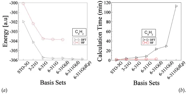
28 CHAPTER 3. CALCULATION FOR VIBRATIONAL FREQUENCIES timization calculation for both HF and DFT methods on the same figure in order to understand the effect of their usages. Figs. 3-1, to 3-5 show the results of opti-mization calculation which are clearly distinguishable from each other. In those figures the total ground state energy as a function of basis sets are plotted.In order to compare the cost effectiveness the total calculation time as a function of basis sets are also plotted. We present an analysis on our calculation result in the next sub-section.

(a) (b).

Figure 3-1: Shows energy (a) of C8H2 molecule and the calculation time (b) as a function of basis sets for both DFT and HF methods. The energy (vertical axis of left side figure), expressed in hartree, refers to the total energy of the molecule at ground state. The calculation time (vertical axis of right side figure, expressed in minutes, refers to the total time of calculation spent for both geometry optimization plus frequency calculation. The optimized energy (lowest energy) of C8H2 molecule is about -303.858 hartree and -305.897 hartree obtained at HF and DFT methods respectively. In the case DFT calculation we used more larger basis sets to get more accurate results whereas we did not do the same for HF method. The reason is explained in the text.

(36)

3.1. OPTIMIZED STRUCTURES OF POLYYNES 29

(a) (b)

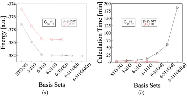
Figure 3-2: Shows optimized data for the molecule C10H2. The explanation of this figure is similar to the above Fig.3-1. The total ground state energy of C10H2 molecule is about -379.539 hartree and -382.079 hartree obtained by HF and DFT methods respectively.

Fig. 3-2: figure/opt-energy-c10h2-DFT-HF.eps, figure/opt-time-c10h2-DFT-HF.eps Fig. 3-3: figure/opt-energy-c12h2-DFT-HF.eps, figure/opt-time-c12h2-DFT-HF.eps

(37)

30 CHAPTER 3. CALCULATION FOR VIBRATIONAL FREQUENCIES

(a) (b)

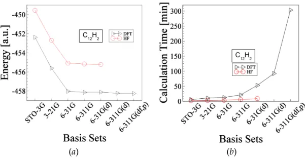
Figure 3-3: Shows optimized data for the molecule C12H2 The explanation of this figure is similar to the above Fig.3-1. The total energy of this molecule at ground state is about -455.219 hartree and -458.26.079 hartree obtained by HF and DFT methods respectively.

(38)

(a) (b)

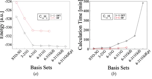
Figure 3-4: Shows optimized data for the molecule C14H2 The explanation of this figure is similar to the above Fig.3-1. The total ground state energy of this molecule is about -530.90 hartree and -534.44 hartree obtained by HF and DFT methods respectively.

Fig. 3-4: figure/opt-energy-c14h2-DFT-HF.eps, figure/opt-time-c14h2-DFT-HF.eps Fig. 3-5: figure/opt-energy-c16h2-DFT-HF.eps, figure/opt-time-c16h2-DFT-HF.eps

(39)

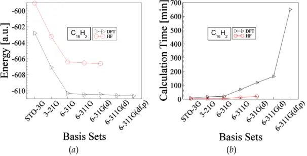
(a) (b)

Figure 3-5: Shows optimized data for the molecule C16H2 The explanation of this figure is similar to the above Fig.3-1. The total ground state energy of this molecule is about -606.58 hartree and -610.626 hartree obtained by HF and DFT methods respectively.

(40)

3.1.1 Analysis of results of optimization calculation

The left side of all the Figs. 3-1 to 3-5 show that the total energy (in hartree) decreases rapidly with larger basis sets up to 6-31G. The use of further more larger basis sets does not affect so much in the case of HF method whereas in the case of DFT method it affects a little. In the case of DFT method we run the program for more larger basis sets whereas we did not do that of HF method because after each optimization calculation we immediately calculated vibrational frequency with this recently obtained optimized structures. We repeated the procedure for both HF and DFT method using the basis sets with the order of STO-3G, 3-21G, 6-31G, 6-311G, and 6-31G(d). We examined the frequency data and found that there is a good tendency of reproduction of experimental results in the case of DFT method whereas HF method did not show such positive tendency that’s why we give up to use further larger basis sets for HF calculation. On the other hand we continue to increase basis sets upto 6-311G(df,P) for DFT calculation even though these calculations were far expensive than the others as shown by the right side of all Figs. 3-1 to 3-5. The vertical axes representing calculation time (in minutes) refer to the total time duration of optimization calculation plus frequency calculation. We can easily see that the use of lager basis sets costs big difference between DFT and HF method. Hence HF method seems to be more expensive than the DFT method. In general we know that the HF method should be more expensive than the DFT one because, in the case of HF method, the solution for electronic wave function i.e. Slater determinant would take longer time. In fact, in general this concept is true, but in particular the expense may depend what type of DFT functional is used. It is well known that the B3LYP functional is expensive over other pure LDA or LSD or pure GGA type functional. Another reason we can here highlight is that for larger basis sets we encountered SCF convergence problem. That is for larger basis sets sometimes the program terminated abnormally showing some error messages which would related with SCF convergence. In order to solve this problem, in most

(41)

34 CHAPTER 3. CALCULATION FOR VIBRATIONAL FREQUENCIES cases, we used forced convergence method with the help of keyword SCF = QC. This keyword, usually, drive the program to the very large number of SCF cycles to get the convergence. We did not plot here the optimized bond lengths in a similar way to energy and time, because we found that the bond lengths did not vary too much for both these methods. We have included the data ,tabulated form, for the optimized bond lengths in the appendix section of this thesis. As we can not have any exact values for C-H or C-C or C ≡ C bonds, because it is well known that bond structures are affected by the molecular environment itself. Nevertheless, we can compare our obtained optimized bond lengths with some other reference values in which the authors relied on that structures. For example, Panaghiotis

et. al.(2003) and Karpen (1999) used the optimized bond lengths for diacetyle are

C − H = 1.0667Å, C − C = 1.3819Å, C ≡ C = 1.2340Å and C − H = 1.0623 Å, C − C = 1.3692Å, C ≡ C = 1.2202Å respectively. Our main concentration, hence, to reproduce the experimental vibrational frequency using a suitable optimized structure. In the next section we will show that it is also needed to take larger basis sets for DFT to reproduce experimental results more closely.

3.2 Calculation results of vibrational frequency

After obtaining the optimized structures of polyynes, we calculated the vibrational frequency on the basis of these optimized structures. The polyynes are linear molecular chain, the number of normal mode of vibration is hence 3n − 5 where n is the number of atoms in the polyyne molecules. As some of the vibrational modes have the possibility to be Raman active, we set our calculation to get Raman activity of each mode of vibration. The following Figs. 3-6, 3-7 show the vibrational frequencies of different lengths of polyynes.

We can see from the Figs. 3-6 and 3-7 that the use of larger basis sets in DFT

Fig. 3-6: figure/alpha-dft-sto-631gd-notscaled.eps, figure/alpha-hf-sto-631gd-notscaled.eps Fig. 3-7: figure/beta-dft-sto-631gd-notscaled.eps, figure/beta-hf-sto-631gd-notscaled.eps

(42)

3.2. CALCULATION RESULTS OF VIBRATIONAL FREQUENCY 35

(a) (b)

Figure 3-6: (a) Shows vibrational frequencies of polyynes on the basis of differ-ent optimized geometries. These bands are attributed as α- bands as these are the strongest peaks observed experimentally. The graph represented by up-triangle are the experimental values whereas all other values are obtained through DFT(B3LYP) calculation.These graphs show a positive tendency to reproduce experimental re-sults. (b) Illustrates the similar phenomena as of (a), the difference is the calculation is carried out by HF method and the graph do not show good tendency to reproduce experimental results.

calculation has a tendency to reproduce the experimental data i.e. both α−bands and β− bands. On the other hand, in the case of HF method it seems not to reproduce the experimental results with good agreement. In this stage we used a scaling factor 0.9644 for the basis 6-311G for DFT(B3LYP). The effect of using scaling factors are represented by the following Fig.3-8.

From Figs.3-8 we see that α− bands are almost reproducible with the use of such scaling factor 0.9644 but the β-bands show slightly mismatched in nature. In order to have a good result for β− bands as well, we further continue to use more larger basis sets that is we added polarization functions for both C and H atoms. The optimized structures of polyynes due to these basis sets i.e. 6-311G(d), 6-311G(df,p) have been tabulated in the appendix section. The α- and β-bands corresponding to these two different optimized geometries are shown in the following Figs. 3-9.

(43)

(a) (b)

Figure 3-7: (a) Shows the vibrational frequencies which are attributed as β- bands as they are the second highest strongest intense peak observed experimentally. The graph represented by up-triangle are the experimental values whereas all other values are obtained through DFT(B3LYP) calculation. (b) Illustrates the similar phenomena as of (a) obtained by HF method and the graphs do not show good tendency to reproduce experimental results.

Finally, the results of DFT(B3LYP) with 6-311G(df,p) were scaled by a suitable scaling factor 0.961. The scaled results for vibrational frequencies are shown in Figs.3-10.

3.2.1 Analysis of vibrational frequency

In order to make an analysis on the vibrational frequency, we review the definition of α- and β- modes. The actual definition of these mode is given in the literature by Tabata et al. [27]. Both of them arise from bond stretching mode of vibration and they appear at higher frequency region. Between the two modes one which has highest Raman scattering activities is considered as α-mode and the second highest Raman scattering activities refers to the β-mode. These two modes are resemble with experimental Raman shifts at α- and β-bands. The α- and β- mode of

Fig. 3-9: figure/alpha-dft-largest-basis-notscaled.eps, figure/beta-dft-largest-basis-notscaled.eps

(44)

(a) (b)

Figure 3-8: (a) Shows α- bands of polyynes obtained by DFT(B3LYP) with 6-311G basis sets scaled by 0.9644 and (b) shows β- bands of polyynes obtained by DFT(B3LYP) with 6-311G basis sets scaled by 0.9644.

vibrational displacement is shown in Fig. ??. It can be noticed here that the center of symmetry of C8H2, C12H2 and C16H2 molecules is C-C (single) bond whereas that of the C10H2and C14H2is C≡ C (triple) bond. So we can classify the into C2nH2 and C2n+2H2group.

We also plot here frequencies for all the 3N − 5 normal mode of vibrations to understand clearly the localizations of these modes. Fig. 3-13(a) shows all normal mode of vibrations for all of our polyynes samples. The frequency region around 2100-2300 cm−1_{(not scaled value) are responsible for α- and β-bands because this} range of frequency arise ,typically, due to the C≡ C bonds stretching mode. The higher frequency region above 3000 cm−1_{is due to the C-H bond stretching mode} which does not vary with the length of polyynes.

We see from Fig. 3-13(b) that the nature of α-mode is quite linear that is frequency decreases with lengths of polyynes almost linearly. On the other hand β-modes

Fig. 3-11: figure/c8h2-alpha-mode-displacement.eps, figure/c10h2-alpha-mode-

displacement.eps,figure/c12h2-alpha-mode-displacement.eps,figure/c14h2-alpha-mode-

displacement.eps,figure/c8h2-beta-mode-displacement.eps,figure/c10h2-beta-mode-displacement.eps, figure/c12h2-beta-mode-displacement.eps,figure/c14h2-beta-mode-displacement.eps

(45)

(a) (b)

Figure 3-9: (a)Shows the vibrational frequencies for α- mode (upper two graphs) which are compared with the experimental Raman shifts α-bands (triangle-up black color) [27] and (b) shows the vibrational frequencies for β-mode (upper two graphs) which are compared with the experimental Raman shifts β-bands (triangle-up black color) [27]. The calculated results are obtained by DFT(B3LYP) with 6-311G(d) and 6-311G(df,p) basis sets. The data are not scaled.

show some oscillating nature but eventually decreasing with lengths of polyynes. Up to C14H2 β-modes appear at lower frequency than that of α-modes but in the case of C16H2β-mode appears at higher frequency region than that of α-mode. We can make a conclusion here about the higher frequency of vibration of α-modes by stating that as the molecular vibration occurs at the central region hence it may require more energy to vibrate. Similarly, we can say that the vibrational frequency of beta modes are comparatively lower as the molecular vibration occur at the terminal region which may require less energy to vibrate.

Now in order to explain the linearly frequency decreasing nature of alpha modes we can consider the atomic displacements at the terminal (end) regions. As we already mentioned that in the case of alpha mode the vibration occur mainly at the central region and if we examine at the terminal region deeply we can see that the displacement of atoms at the terminals are very small that they can be thought as the fixed end of a spring. That means the nodes of vibration occur at the terminals.

(46)

(a) (b)

Figure 3-10: (a) Shows the vibrational frequencies for α- mode (triangle-down red color) which are compared with the experimental Raman shifts α-bands (triangle-up black color) [27] and (b) shows the vibrational frequencies for β-mode (open circle red color) which are compared with the experimental Raman shifts β-bands (triangle-up black color) [27]. The calculated results are obtained by DFT(B3LYP) with 6-311G(df,P)basis sets for both cases. The data are scaled with 0.961

Hence with the increase of length of polyynes (increasing number of atoms in polyynes) the distance between two nodes are increasing which in turn decrease the frequency of vibration.This phenomena can be explained by the Fig. 3-12.

The β−modes are quite complicated because they show oscillation behavior in decreasing frequency with increasing molecular size. We made an explanation in describing this oscillation nature by grouping polyyne molecules into two groups. The group H(C ≡ C)2nH is formed with polyynes whose center of symmetry is single bond and the other group H(C ≡ C)2n+2H is formed with polyynes whose center of symmetry is triple bond. We see that in the case of H(C ≡ C)2nH the nature of molecular vibration is such that there are contributions from both single and triple bonds that result this group to posses higher frequency than the group H(C ≡ C)2n+2H in which there is no contribution from single bonds.

Fig. 3-12: figure/alpha-mode-explanation.eps

(47)

(a) (e)

(b) ( f )

(c) (g)

(d) (h)

Figure 3-11: (a - d) Show the vibrational displacements of α-modes of C2nH2; n=4 . . . 7. Figs (e - h) show the displacements of β-modes of vibration for the same molecules. For α-modes of vibration the displacements occur at the central region i.e. around the center of symmetry while the displacements corresponding to β-mode of vibration appear at terminal region.

In order to understand the vibrational mode in the view of molecular symmetry and group theory we plot the 3N − 5 normal modes of vibration as shown in Fig.3-14. We can see that among four vibrational symmetry modes e.g. Πg, Πu, Σgand Σu, the higher frequency regions are due to the vibrational modes Σgand Σu. The other two modes of vibration i.e. Πgand Πuappear mostly at the lower frequency region. We can also see that at the top region (above 3000 cm−1_{) on the plot frequency does} not vary much with the length of polyynes. The vibration of H atom at the end of the molecules is responsible for this higher frequencies because of its light weight.

(48)

Figure 3-12: Shows an schematic explanation of linearly frequency decreasing nature of α-modes. It can be seen that the two terminals of polyyne molecule are thought to be fixed ends of a spring because the displacements of terminal atoms from their equilibrium are negligible. Hence with the increase of molecular lengths the distances between two nodes are increasing i.e. increasing wavelengths.

(49)

(a) (b)

Figure 3-13: (a) Shows the 3n − 5 normal mode of vibrations obtained by DFT(B3LYP) with 6-311G(df,p). The frequency region around 2100 − 2300cm−1 are responsible for α- and β-bands. The higher frequency region above 3000 cm−1 is due to the C-H bond stretching mode which almost constant with the length of polyynes (b) Shows the expanded view of the frequency region 2100-2300 cm−1 (not scaled)

(50)

Figure 3-14: Shows the 3N − 5 normal modes of vibrations of different lengths of polyynes in the view of molecular symmetry. Σg, Σu modes are dominating at higher frequency region. Both α− and β− modes are belong to the Σgvibrational mode. We can also see that at the top region (above 3000 cm−1_{) on the plot frequency} does not vary much with the length of polyynes. The vibration of H atom at the end of the molecules is responsible for this higher frequencies.

(51)

(52)

Chapter 4 Excited States Energies and NMR

Calculations

In this chapter we will show our calculated results of singlet excited states energies and NMR results for chemical shift (δ) of a series of polyynes i.e. (C ≡ C)2n; n = 4 . . . 8. The calculation methods are described in the chapter 2.

4.1 Calculated results of excited states energies

The following Fig. 4.1 shows the calculation results for singlet excited states energies of polyynes (C ≡ C)2n; n = 4 − 8. We set our calculation to predict the singlet excited states energies of first three states. Here we can see clearly the dependence of calculation results on the choice of basis sets. The figures also shows that the energies decrease with the length of the molecule. This is result is similar with the vibrational calculation result in chapter: 3 section: 3.2 where it is noticed that the vibrational frequencies of Raman active modes decrease with molecular size (length). This is obvious because vibrational features of Raman active modes specially the resonance condition of Raman scattering is closely related with excited states energies.

(53)

46 CHAPTER 4. EXCITED STATES ENERGIES AND NMR CALCULATIONS

Figure 4-1: Shows singlet excited states energies of a series of polyynes at the different optimized structures. The calculation is performed using CIS method

In this calculation we did not try to reproduce any experimental data for the excitation energies of bared polyynes rather we tried to predict the excitation en-ergies for the hybrid system polyynes@SWNT. It has been reported in the litera-ture [36] that the intense resonant phenomena for the systems C10H2@SWNT and C12H2@SWNT observed at laser energies near around 2.1 electron volts which is shown at the bottom of Fig. 4.1. We see that the excited states energies of polyynic P bands ,while polyynes are trapped inside SWNT, are lower than that of bare polyynes. This is consistent because as bare polyynes are pure one dimensional structures hence the exciton binding energies are higher than polyynes are inside SWNT, because in this case the purity of one-dimensionality of the hybrid system (polyynes@SWNT) is reduced. Now, in answering the question “why pure one dimensional structures possess higher binding energy? ”, we can phenomenologi-cally mention that in the case of one dimensional structure the degree of freedom of electron-hole pair (exciton) is much lower than the multi-dimensional structures.

(54)

4.2. CALCULATED RESULTS OF NMR 47 Hence electron-hole pair can not escape each other in any arbitrary direction hence bound tightly.

For this hybrid system (polyynes@SWNT) it could be expected that the elec-tronic transitions through the optical absorption can take place from SWNTs to excited states of polyynes which would result a high intense of Raman signals. In our calculated results we see that the excited states energies for C10H2 and C12H2 range from2.75 to 3.5 eV and 2.65 to 2.95 eV respectively. In order to interpret our results, actually, we need to consider two main things: one is to consider more accu-racy of calculation by considering more configuration of excited states of polyynes and secondly we need to consider the excitonic picture of polyynes or the exitonic picture of the hybrid system. For this moment we can say that our calculation for excited states is not complete yet rather this is a first step to consider the excitonic feature of the hybrid system.

4.2 Calculated results of NMR

Chemical shift, which is independent of external magnetic field strength and op-erating frequency of NMR spectrometer, is an important information for NMR calculation. It is measured with the help of a reference value of a standard sample. In our calculation we use the reference values that is the chemical shift values of 1_{H and} 13_{C of tetramethylesilane (TMS) as the standard reference which are} ob-tained by the same method and level of calculation. DFT (B3LYP) and the basis 6-311G(2d,p) is used to optimize the structure and NMR calculation is performed by GIAO (Gauss Independent Atomic Orbital) method.

We can see from the Table 4.1 that in most cases (both in experimental and calculation) the coupling between 1_{H and} 13_{C nuclei becomes weaker with the} distance between them. But for some other nuclei, even though, those are far

Fig. 4-2: figure/chemical-shift-H.eps, figure/chemical-shift-c8h2.eps Fig. 4-3: figure/chemical-shift-c10h2.eps, figure/chemical-shift-c12h2.eps