数学と化学の学際共同研究と福井プロジェクト

(1)

有本茂^*1

Massoud Amini

^*2

Hao Chen

^*3 福田信幸^*4

Joseph E. LeBlanc

^*5 村上達也^*6 成木勇夫^*7

Mark Spivakovsky

^*8 竹内茂^*9

Keith F. Taylor

^*10

Hong Yi Wong

^*11 山中聡^*12 横谷正明^*13

Peter Zizler

^*14

Mathematics and chemistry

interdisciplinary joint research and the Fukui Project XXII

Shigeru ARIMOTO, Massoud AMINI, Hao CHEN, Nobuyuki FUKUDA, Joseph E. LEBLANC Tatsuya MURAKAMI, Isao NARUKI, Mark SPIVAKOVSKY, Shigeru TAKEUCHI

Keith F. TAYLOR, Hong Yi WONG, Satoshi YAMANAKA, Masaaki YOKOTANI and Peter ZIZLER

This is the 22nd part of the series of articles that records and further develops essentials of the Mathematics and Chemistry Interdisciplinary Symposium 2013 Tsuyama, whose main themes were symmetry, periodicity, and repetition. The symposium was held on April 5th and 6th in Tsuyama city, Okayama, Japan, in conjunction with the Fukui Project and was devoted to the memory of the late Professor Kenichi Fukui (1981 Nobel Prize) who initiated the project. The present series also provides challenging cross-disciplinary problems which are directly related to the Fukui conjecture and to recent carbon nanotube research. Some of these problems are formulated using mathematical language not well known among chemists despite the importance of these notions in elucidating additivity and high-speed asymptotic phenomena in molecules having many repeating identical moieties. Some problems are formulated in terms of Fourier analysis connected to the theory of analytic curves, others are formulated in connection with the Science-Art Multi-angle Network (SAM Network) Project, which seeks to bridge Science and Art (visual, audial, and conceptual) for a creative collaboration, and is an important part of the Fukui Project.

Key Words: the Fukui conjecture, Memoir of Prof. K. Fukui, Unique factorization domain (UFD), Carbon nanotube, Fourier analysis

I Introduction

10. Proof of the Off-diagonal Asymptotic Linearity Theorem X_(1) simple version

without using the Piecewise Monotone Lemmas

Shigeru Arimoto, Massoud Amini, Hao Chen Nobuyuki Fukuda, Isao Naruki, Mark Spivakovsky Shigeru Takeuchi, Keith F. Taylor, Satoshi Yamanaka

Masaaki Yokotani and Peter Zizler

In this section, we prove a simple version of the Off-

原稿受付平成29年9月21日

＊1, ＊12, ＊13 総合理工学科＊4 総合理工学科非常勤講師

＊2 Dept. of Math.Tarbiat Modares University, Iran

＊3 Dept. of Fund.Ed., Dalian Neusoft University of Information, China

＊5 School of Integrated Studies, Pennsylvania College of Technology USA

＊6 富山県立大学工学部・医薬品工学科

＊7 立命館大学理工学部・数学物理学系・数理科学科・元教授

＊8 CNRS and Institute de Mathématiques de Toulouse, France

＊9 岐阜大学教育学部・数学科

＊10 Dept. of Math. and Stat., Dalhousie University, Canada

＊11 School of Communication, Arts and Social Sciences, Singapore Polytechnic, Singapore

＊14 Dept. of Math., Phys., and Eng., Mount Royal University, Canada

－25－

(2)

diagonal Asymptotic Linearity Theorem (OALT-X_(1) AC(I) version: OALT-0.1) without using any version of the Piecewise Monotone Lemma (PML) (see Refs. [1-5] and references therein). Since we deal with elements {AN}  X_(q) with q = 1, the proof is easier than in the general case in which the block-size q of block matrix AN is greater than 1. If q = 1 then AN is not a block matrix but just an NN matrix, and AN is diagonalizable for all N >> 0, according to the definition of the alpha space X_(1). The crux of the proof is to use the fact that both (AN) and P_N^s are simultaneously diagonalizable by the same unitary matrix UN, hence the product (AN) and (AN)P_N^s is diagonalizable by the same unitary matrix UN. The situation is similar in the general case of X_(q) in which

(AN) and P_N^s Iq are simultaneously block- diagonalizable by the same unitary matrix UNIq, hence the product (AN)(P_N^sIq) is block-diagonalizable by the same unitary matrix UNIq. Before proceeding to the proof, the reader is asked to recall the following fundamentals [1- 5]:

Definition 1. Let S1 and S2 be nonempty subsets of . A function f: S1  S2 is said to be nondecreasing if x1 ≤ x2

implies f(x1) ≤ f(x2) for all x1, x2  S1. A function f: S1  S2

is said to be nonincreasing if x1 ≤ x2 implies f(x2) ≤ f(x1) for all x1, x2  S1. A function f: S1  S2 is said to be monotone if it is either nondecreasing or nonincreasing.

Let a, b  with a < b and let I = [a, b]. A function f: I

 is said to be piecewise monotone if there exists a finite partition

a = x0 < x1< ... < xn = b (n  ⁺) (2.1) of the interval I such that the restriction f | [xi-1, xi] is monotone for all i  {1,..., n}. In this case, f is said to have n-partition of monotonicity.

A real-valued function on a subset S  is called real analytic on S if it is the restriction to S of a function which is real analytic on some open set O  S.

Let a, b  with a < b, let I = [a, b]. The symbol C(I) denotes the set of all real-valued continuous functions on I.

A function  : I  is said to be absolutely continuous on I if, given any  > 0, there exists a  > 0 such that for every finite system of pairwise disjoint subintervals (a1, b1), (a2, b2), ..., (an, bn)  [a, b],

1 n



k ^(b^k^{– a}^k^{) < }

implies

1 n

k



^|(b^k^{) – (a}^k)| < .

The symbol AC(I) denotes the set of all real-valued absolutely continuous functions on I. If f is a real-valued function on I and if S is a subset of I, then f | S denotes the function f restricted to S. In this article, the symbols C(I) and AC(I) used in Refs. [1-5] are often represented by C[a, b] and AC[a, b] respectively. The following Proposition 1 is fundamental in the present section:

Proposition 1. Let a, b, c  with a < c < b. The following statements are true:

(i) If f  C[a, b], f | [a, c] AC[a, c], f | [c, b] AC[c, b], then f  AC[a, b].

(ii) If f  AC[a, b] is a monotone non-decreasing function and if g  AC[f(a), f(b)], then g  f  AC[a, b].

Proof. The conclusions easily follow from the definition of absolutely continuous functions. //

Note 1.

It is easy to check that

(i) The derivative f of real analytic function f

 AC(I) is real analytic.

(ii) The set of zeroes of a real-analytic function f  AC(I) on the closed interval I is either empty, a discrete (and hence a finite) set, or the entire domain I.

(iii) Any real analytic function f  AC(I) is piecewise monotone.

(iv) The functional space AC(I) forms an algebra with respect to the linear operations and the multiplication of functions.

Note 2. For the definitions of X_(1) and the FS map, the reader is respectively referred to Eq. (C.1) and Eq.

(C.8) in the Appendix to Part XX of this series. See also Refs. [8,9]. The matrix F() appearing in the following Theorem 1 is a 1  1 real-symmetric matrix, that is, a real number, for every    . The matrix F() is sometimes called the F-theta matrix associated with the sequence {AN}. In Ref. [9], for the general case in which {AN}  X_(q) with q  ⁺, it was proved that all the eigenvalues of the q  q real-symmetric matrix F() are contained in the interval I for all    .

Theorem (OALT-X_(1) AC(I) version: OALT-0.1). Let s  , let {AN}  X_(1), and let I be a closed interval which contains all the eigenvalues of AN for all N 

－26－

+ . Then,

(3)

for any   AC(I), there exists an s()  such that Tr[((AN))P_N^s] = s()N + o(1) (1) as N  . Moreover, s() is represented by the integral:

s() = ²

0

1 exp( ) ( ( ))

2 ^ is  F  d





^,

where F is the FS map associated with the sequence {AN}.

Proof. Assume that

AN = ^v _N^j _j

j v

P Q





 (2) for all N >> 0. Then, the FS map associated with {AN} is given by:

F() = ^v



^exp( ⁾



j j v

ij Q



 . (3) Let DN denote the N  N diagonal matrix defined by D: diag exp(i^{2 1}), exp(i^{2 2}), , exp(i² N)

N N N

  

 

 

  . (4)

Recall the fact that the matrix PN is expressed in terms of a unitary matrix UN and a diagonal matrix DN:

PN = UNDNU_N^¹. (5) Thus, plugging (5) into (2), and using a fundamental property of Kronecker product: (A  B)(C  D) = (AC)

(BD), we have

AN = (UNI1) ^v _N^j _j

j v

D Q



 

  





^(U^N^I¹⁾^¹

= UN v

j

N j

j v

D Q



 

  





^U^N^¹^, and hence

 (AN) = UN 1

exp 2

N v k j

j v

ij k N Q

 

 

     

     

    





^U^N^¹⁽⁶⁾

for all N >> 0, where

1 N

k denotes the direct sum of 1 1 matrices indexed with k, which implies that the matrix in (6) enclosed by the brackets [ ] is an NN diagonal matrix.

On the other hand, we have

s

PN = U_N D_N^s U_N^¹

= UN 1

exp 2

N k

i sk N





  

   

 UN^¹. (7) Thus, by (3), (6) and (7), we have, for all N >> 0,

Tr[((AN))P_N^s]

= Tr[UN 1

2 2

N exp

k

i sk k

N F N

  



     

       

 UN^¹]

= Tr 1

2 2

N exp

k

i sk k

N F N

  



     

       

 

=

1 N



k ^^^^exp^ⁱ²^_N^sk^^{ }  ^ ^F^²_N^^k^^^^

=

1 N



k ^^^cos^²^_N^sk^^{ }  ^ ^F^²_N^^k^^^ + i

1 N



k ^^^^^sin^²^_N^sk^^{ }^{ } ^ ^F^²_N^^k^^^^^ (8) Note that Q__j Q_j for all   v j v by the definition of the alpha space X_(1). Hence, one easily sees that

( )

F is a real analytic function because the imaginary part vanishes and the real part is a linear combination of trigonometric functions cos j. We infer that the function

( )

F is piecewise-monotone and continuously differentiable, and hence absolutely continuous on [0, 2].

(Note: Continuously differentiable functions, or C¹ functions on a closed interval are Lipchitz functions.

Lipchitz functions on a closed interval are absolutely continuous functions. Thus, the functions  coss and sins are both absolutely continuous functions on [0, 2].)

Recalling Proposition 1 and the fact that the product and sum of absolutely continuous functions are absolutely continuous functions, we easily see that for any   AC(I), the function

1

(cos ) ( ( ))

q

m

s F

   





 (9)

is absolutely continuous on [0, 2 ] and that for any   AC(I), the function

1

(sin ) ( ( ))

q

m

s F

   





 (10)

is absolutely continuous on [0, 2]. Now either Zizler’s Theorem, or Theorem #1 reproduced below easily implies that

Tr[((AN))P_N^s] =

－27－

(4)

2 0

1 exp( ) ( ( ))

2 ^ is  F  d N





+ o(1) (11)

as N  .

The conclusion follows. [Note that the sequence Tr[((AN))P_N^s] is a real sequence, hence the imaginary part of the above integral must vanish, thus we have in fact:

2 0

1 exp( ) ( ( ))

2 ^ is  F  d





= ²

0

1 (cos ) ( ( ))

2 ^ s  F  d





^,

and hence

Tr[((AN))P_N^s] = ²

0

1 (cos ) ( ( ))

2 ^ s  F  d





^N

+ o(1) (12)

as N  . This formula is used in a computer experiments

given below.] //

Theorem 1. Let a, b  with a < b, let x(N, k) := a + (b

 a)k/N, and let f  AC[a, b]. Then, we have

1 N



k f(x(N, k)) = (1/(b  a))( ^b ( )

a f  d



^{)N +}

(1/2)(f(b)  f(a)) + o(1) (13) as N  .

Proof. This was first proved in [6] by using the ALT. //

Note: The above Theorem 1 directly follows from Zizler’s Theorem which was proved by Peter Zizler for the first time in Section 3 of [7].

Computer experiments:

Let

2 1 1

1 2 1

1 2 0

,

0 2

2 1 1 2 1

1 1 2

N

A

 

 

  

 

  

 

 

 

  

   

 

  

 



 





and let(x) = x^{1/ 2}, then we have F() =



exp( ( 1) )i  



Q_1



exp( (0) )i 



Q0



exp( (1) )i 



Q1



=



exp( ( 1) ) ( 1)i  



 



exp( (0) ) 2i 





exp( (1) ) ( 1)i 



 

=



^{cos(( 1) )}  isin(( 1) ) ( 1) 





 

2 cos(( 1) ) isin(( 1) ) ( 1)

     

= 2 2 cos = 4sin² 2

 . Hence,

Tr[((AN))P_N^s] = ²

0

1 exp( ) ( ( ))

2 ^ is  F  d N





^{+ o(1)}

= ²

0

1 (cos ) ( ( ))

2 ^ s  F  d





^{N + o(1)}

= ²

0

1 (cos ) 2sin 2 ^ s 2 d





^{N + o(1)}

= ²

0

1 (cos ) sin

s 2 d

   





^{N + o(1)}

=

0

2 (cos )sin

s 2d

   





^{N + o(1)}

= ₂

4 1 4s



 N + o(1) (14)

as N  .

We remark that the above number ₂ 4 1 4s



 of the slope of the asymptotic line was derived through elementary trigonometric calculations and the derivation is omitted here. Using Graphing Calculator, one can numerically check the Eq. (12). For the case of s = 0, the above asymptotic formula has been well known since the earlier time when the investigation of the Fukui Conjecture was started.

We provide in what follows (i) the Graphing Calculator code to numerically check Eq. (14) and (ii) the MATLAB code that produced the Matrix art pictures (AN) given in Figs1 in the following pages.

Graphing Calculator code:

With the above function appearing in the Fukui Conjecture, given any integer s, this program draws the OALT asymptotic line in red, and the actual plot in blue for the example of Cyclic Liner Chain

－28－

(5)

matrix A_N. (Aug 24, 2017)

In the editable file, one can click the value of integer s at the lower right corner and change its value.

MATLAB code:

MATLAB code that created the original picture of  (A

N

) with N = 50. The pictures were later edited by using a photo editing software.

% OALT Matrix Art % Aug 24, 2017

function f = MA(N)

M = 2*((P(N))^0) - P(N)' - P(N);

A = (M*M)^(1/4);

axis square figure

surf(real(A));

function P = P(N);

% This function creates matrix P(N) with N

% = 1, 2, ...

%

% For example:

% % P(1) = % % 1 % % P(2) = %

% 0 1 % 1 0 %

% P(3) = %

% 0 1 0 % 0 0 1 % 1 0 0 %

% P(4) = %

% 0 1 0 0 % 0 0 1 0 % 0 0 0 1 % 1 0 0 0

for i = 1:N for j = 1:N

if i - j == -1 P(i,j) = 1;

else

P(i,j) = 0;

end end end

P(N,1) = 1;

－29－

(6)

MATLAB Matrix Art:

－30－

(7)

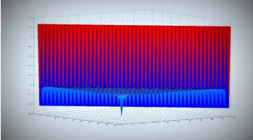
Figs 1. Matrix art of (A50), with entries plotted to the z axis direction. Observe that the peak of this figure is approximately

2

4 1 4 0



  = 1.273 … , and the first off-diagonal entries are approximately ₂ 4 1 4 1

  =



0.424 … , and note that the sequence

2

4 1 4 s



  converges to 0 monotonously from below.

References

[1] S. Arimoto, M. Spivakovsky, K.F. Taylor, and P.G. Mezey, Proof of the Fukui conjecture via resolution of singularities and related methods. I, J. Math.

Chem. 37 (2005) 75-91.

[2] S. Arimoto, M. Spivakovsky, K.F. Taylor, and P.G. Mezey, Proof of the Fukui conjecture via resolution of singularities and related methods. II, J.

Math. Chem. 37 (2005) 171-189.

[3] S. Arimoto, Proof of the Fukui conjecture via resolution of singularities and related methods. III, J. Math. Chem. 47 (2010) 856-870.

[4] S. Arimoto, M. Spivakovsky, K.F. Taylor, and P.G. Mezey, Proof of the Fukui conjecture via resolution of singularities and related methods. IV, J.

Math. Chem. 48 (2010) 776-790.

[5] S. Arimoto, M. Spivakovsky, E. Yoshida, K.F. Taylor, and P.G. Mezey, Proof of the Fukui conjecture via resolution of singularities and related methods. V, J. Math. Chem. 49 (2011) 1700-1712.

[6] S. Arimoto, The Second Generation Fukui Project and a New Application of the Asymptotic Linearity Theorem, Bulletin of Tsuyama National College of Technology, 52 (2010) 49-56.

[7] S. Arimoto, M. Amini, N. Fukuda, J.E. LeBlanc, T. Murakami, I. Naruki, M. Spivakovsky, S. Takeuchi, K.F. Taylor, S. Yamanaka, M. Yokotani, and P.

Zizler, "Mathematics and Chemistry Interdisciplinary Joint Research and the Fukui Project XIV", Bulletin of National Institute of Technology, Tsuyama

College 58 (2016) 35-39.

[8] S. Arimoto and G.G. Hall, Integral Representation of a Fundamental Functional for the Study of the Zero-Point Vibrational Energy of Hydrocarbons and the Total Pi-Electron Energy of Alternant Hydrocarbons, Int. J. Quantum Chem. 46 (1992) 612-635.

[9] S. Arimoto, New proof of the Fukui conjecture by the Functional Asymptotic Linearity Theorem, J. Math. Chem. 34 (2003) 259-285.

－31－