1. Introduction
Reconstruction of the images of nuclear medicine such as single photon emission computed tomography (SPECT), positron emission tomography (PET), etc. has been performed by using the filtered back projection (FBP) method, the ordered subset expectation maximization (OS-EM) method and the maximum likelihood expectation maximization (ML- EM) method. The use of such an OSEM method that is a successive, approximate-image reconstruction method, etc. has been recently increased. This may be attributed to reduction of streak artifacts from high density areas and the easiness of building attenuation correction, scatter correction, collimator aperture correction, etc. into reconstructive soft- wares[1-4]. In recent years the OESM method has been widely used for clinical purposes, and many
studies on the combination of the number of times of iteration and the number of subsets as well as clinical applications have been made. However, very few studies on the use order of subsets have been made[6- 7]. Most recently a successive approximate image reconstruction method has been adopted for the purpose of reducing the exposure level in the image reconstruction of CT[8-10].
We made a study on the use order of subsets by changing the number of subsets, the calculation order of subsets and the number of times of iteration, and report as follows:
2. Materials and Methods
2-1 Software used in image reconstruction and image processing
For image reconstruction in the present study, we used the software compiling each of the following methods by gcc on the Cygwin (Windows XP) that
Seiji Kawamura1), Yuuki Matsutake2), Takeyuki Hashimoto3), Ryuji Ikematsu2), Yasuyuki Kawaji1), Tadamitsu Ideguchi1),
Shigehiro Fukushima4), Naofumi Hayabuchi5)
Summary (Abstract): The OSEM that is a successive, approximate-image reconstruction method has been extensively used for the image reconstruction of SPECT and PET. The OSEM method has very recently been introduced in the image reconstruction of CT, and its clinical application has begun. As the advantage of the OSEM method, reduction of streak artifacts from a high density area and easiness to build attenuation correction, scatter correction, etc. into reconstructive soft-wares have been mentioned. Many studies on the number of subsets and iterations, etc. in the clinical use of OSEM method have been made up to date, but the studies on the use order of subsets have been scarcely made. Thus, we made a study on the use order of subsets by changing the number of subsets and the use order of subsets of the Shepp phantom images as our study’s subject images. We conducted the comparative examination of Shepp phantom images that were reconstructed under a different condition from the original images of Shepp phantom by using visual NMSE method, pro le curves, contrast, etc. As a result, it was thought that, for the use order of subsets, it may be recommendable to construct a subset per each projected data at the greatest elongation.
Keywords: OSEM, MLEM, FBP, subset, iteration
Received. December20, 2011.
Department of Radiological Science,
Faculty of Health Sciences, JUNSHIN GAKUEN University Professor
Study on the use order of subsets in OSEM Method
JUNSHIN GAKUEN University1), Kurume University Hospital2) Yokohama Soei Junior College3) Kyushu University4), Kurume University School of Medicine5)
is a UNIX-like environment, the OSEM method (P5- 070sem_xct.c) that was down-loaded from http://www.
iryo-kagaku.co.jp/frame/03 -honwosagasu/370/370- dl.htme, the MLEM (P5-06mlem_xct.c), the FBP (P5- 04fbp.c), the Shepp phantom (P3-09shepp.pmt) that is a numerical value phantom, and the source code to be used for producing the projected data. Also, by using Prominence processor 3.0 that is software for nuclear medicine image processing, we conducted calculation for the images display of reconstructed image and the normalized mean square error (NMSE).
2-2 Reconstruction of Images
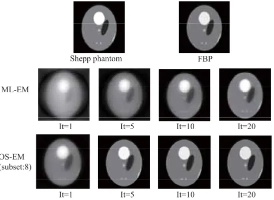
For reconstruction of images, we reconstructed the images using FBP method and OSEM method by making the projected data consisting of 128 directions from the Shepp phantom images Fig. 1. For the image reconstruction, we did not make any image processing such as pre-processed ltering, attenuation correction, etc. At the time of making a reconstruction by OSEM method, we changed the subset from 1to 4, 8 and 16.
At setting of Subset to be 1, we changed the number of iteration to (1, 5, 10, 20). Setting Subset = 1 is equal
to the reconstruction by MLEM method. At setting of Subset at 4, 8 and 16, we changed the number of iteration to (1, 2, 3, 4, 5, 6, 7, 8, 9, 10, 20). Also at setting of Subset at 8, the calculation order of subsets was made at the 2 methods that were shown in the upper section of Fig. 2, namely the original method (1, 5, 3, 7, 2, 6, 4, 8) and the modi ed method (1, 2, 3, 4, 5, 6, 7, 8). The calculation order for setting of Subset at 4 was set to be the original method (1, 4, 2, 3) and the modi ed method (1, 2, 3, 4). Furthermore, the calculation order of Subset at 16 was set to be the original method (1, 9, 5, 13, 2, 15, 4, 12, 3, 14, 6, 11, 7, 10, 8, 16) an the modi ed method (1, 2, 3, 4, 5, 6, 7, 8, 9, 10, 11, 12, 13, 14, 15, 16).
2-3 Evaluation Method
We made a visual evaluation of each reconstructed image. For physical evaluation, we first calculated NMSE, profile curves and mean counts by setting 4 regions of interest (ROI) for each image, and then made evaluation of these indexes. For the computation of NMSE, by using the Shepp phantom images as the standardized ones, and the reconstructed
Shepp phantom FBP
ML-EM
It=1 It=5 It=10 It=20
OS-EM (subset:8)
It=1 It=5 It=10 It=20
Fig. 1 This shows the Shepp phantom images on the upper left hand side and the FBP images on the upper right hand side. It also shows images reconstructed using the MLEM and OSEM methods respectively, in the middle and lower section
images by OSEM method and FBP method as the object images, we employed the below mentioned equation (Equation-1). For the evaluation using the
profile curves, we found the profile curves at the area shown in Fig. 3, and made a visual evaluation.
As shown in Fig. 4 at the upper right, we found the
Fig. 2 This shows the use order of subsets and the images of diff erent subsets and iterations.
Shepp-original X(0.6)
FBP X(0.5997) ( )
Y(0.3333)
( )
Y(0.3333)
OSEM sub=16
OSEM sub=16 sub=16,
iteration=3, modified X(0.5984)
sub=16, iteration=3, original X(0.6)
Y(0.3333) Y(0.3333)
Fig. 3 This shows profi le curves and the diff erent contrasts of the Shepp phantom images, OSEM-modifi ed images and the OSEM-original images.
transition of mean counts by setting 4 regions of interest (ROI 1, 2, 3, 4), to make comparison with the Shepp phantom images and the FBP images.
NMSE= ×100√Σi, jn (p (i, j)Σi, jn q (i, j)−q (i, j))2
Equation 1
q (i, j): Standardized image p (i, j): Observed image
n: Number of pixel in the image
3. Results
3-1 Calculation of NMSE values and graph display
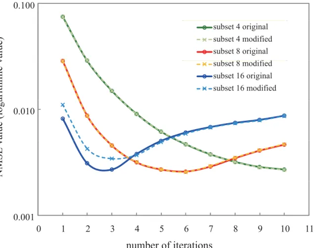
Fig.5 shows the values of NMSE to the differences of subsets (4, 8, 16) and iterations (1, 2, 3, 4, 5, 6, 7, 8, 9, 10). For Subset = 4, both the original and modi ed images showed the smallest value of NMSE = 0.0027
at iteration = 10. For Subset = 8, both the original and modi ed images showed the smallest value of NMSE
= 0.0026 at iteration = 6. For Sabset = 16, both the original and modified images showed the smallest NMSE values of 0.0027 and 0.0034, respectively.
For Subset = 4 and 8, the NMSE values showed nearly same values. For Subset = 16, the original images showed a lower NMSE value, compared with the modified ones, at iteration 1, 2 and 3. (Fig.
5 is the graphed values of NMSE) For Subset = 16, the original images showed a lower NMSE value, compared with the modified ones, at iteration = 1, 2 and 3.
3-2 Comparison of Pro le Curves
Fig. 4 shows the profile curves of the Shepp phantom images and the reconstructed images by FBP and OSEM methods. In the upper left, the Shepp phantom images are shown, in the upper right are the
1 6 1.8 2
M-ROI1
l value
0 8 1 1.2 1.4
1.6 M-ROI2
M-ROI3 M-ROI4 O-ROI1
Pixel
0.2 0.4 0.6 0.8
O-ROI2 O-ROI3 O-ROI4
Subset (4)
2.5 2
e e
Shepp image
1 2 1.4 1.6 1.8 2
M-ROI1 M-ROI2 M-ROI3 1.5
2 O-ROI1
O-ROI2 O-ROI3
Pixel value Pixel value
0.4 0.6 0.8 1
1.2 M-ROI4
O-ROI1 O-ROI2 O-ROI3 0.5
1
O-ROI4 M-ROI1 M-ROI2 M-ROI3
0.2 O-ROI4
0
M ROI3 M-ROI4
Subset (16) Subset (8)
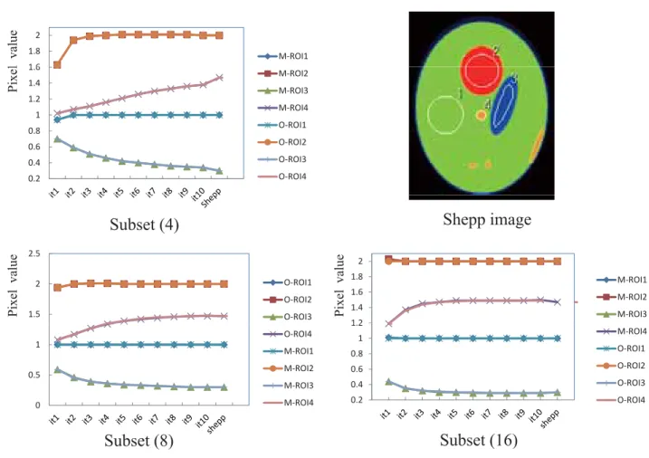
Fig. 4 This shows in a line graph the transition per subset and iteration of pixel values on the upper right hand side, at 4 regions of interest (ROI) that were set in to the Shepp phantom.
FBP images, in the lower left, the modified images are shown for Subset = 16 and at iteration = 3, in the lower right, the original images for Subset = 16 and at iteration = 3 are shown. Each image and pro le curve showed nearly same shapes. The contrast of each image calculated from the highest number of pixels (a) and the lowest number of pixels (b) in the center area of the pro le curves on X-axis and Y-axis was Shepp phantom (0.6, 0.3333), FBP (0.5997, 0.3333), OSEM-modi ed (0.5984, 0.3333) and OSEM-original (0.6, 0.3333), which showed nearly same values. The equation of contrast is set as follows: Contrast = (a-b)/
(a+b).
3-3 Transition of mean pixel values
Fig. 5 shows the transition of mean pixel values per subset (4, 8, 16) and iteration (1, 2, 3, 4, 5, 6, 7, 8, 9, 10), and the mean pixel values per each 4 regions of interest (ROI) of Shepp phantom images. With the advancement of the number of Subnet from 4 to
8, to 16, the pixel values showed convergence to a smaller number of iteration. A similar tendency was also shown in the transition of pixel values in the 2 calculation orders (for original and modi ed images) of Subsets.
4. Discussion
In the ordered subset expectation maximization (OSEM) method, the projected data are divided into several subsets, and the number of pixel is renewed, for each projected data per subset, which is a characteristic of allowing the high frequency component to recover at the time when the number of iteration is small. Although no specific rules on the use order, etc. for the number of Subset and among subsets, it is thought to be good to construct a subset per a projected data at the greatest elongation. In the present study, we examined the influence of the number of subsets or iterations and the use order
0.100
value)
subset 4 original subset 4 modified subset 8 original
b 8 difi d
arithmic v subset 8 modified
subset 16 original subset 16 modified
0.010
value (logaNMSE v
0.001
0 1 2 3 4 5 6 7 8 9 10 11
number of iterations
Fig. 5 This shows in a graph the NMSE values due to the diff erence in subsets and iterations.
among subsets on the reconstructed images.
Fig. 1 shows the images reconstructed by MLEM method, OSEM method and FBP methods as well as the Shepp phantom images. In MLEM method, subset is 1, using all at once the projected data at all angles.
In OSEM method, the projected data are divided into several subsets, and at one iteration the images are renewed many times, resulting in faster convergence.
If we compare the images by MLEM method with those of OSEM in Fig. 1, we are able to understand that OSEM method makes it possible to make the image convergence much faster.
Fig. 2 shows the use order of subsets in the original method and modi ed method for the case of subset = 8 as well as the reconstructed images, but the difference caused by the use order was unable to be visually distinguished. Also, Fig. 5 shows the values of NMSE that were reconstructed under each condition. At subset = 16 and iteration (1, 2, 3), divergences arouse between the original method and the modi ed method, showing that the original method generated lower NMSE values. This may be due to the factors, in which the use order in the original method, compared with that of the modified method, composed the subsets for each projected data made at the greatest elongation. Fig. 5 is the graphed the valuse of NMSE, revealing clearer divergences between the original method and the modi ed method at subset = 16. Thus, despite less number of times of iteration by using the original method, it was shown that the images became more approximate to the Shepp phantom images.
This may contribute to the improvement in reduction of the computation time required for the image reconstruction as well as the improved through-put in the examination by nuclear medicine.
Differences in the shapes and contrasts of profile curves in 4 images shown in Fig. 4 were hardly observed. The use order of 2 subsets that were used from Fig. 5 in the present study did not show any in uence on the transition of pixel counts within ROI.
As seen above, the use order of subsets in OSEM method scarcely influenced the transition of pixel values and the visual evaluation of the images.
However, in the evaluation of NMSE values, at subset
= 16, disvergences in the NMSE values between the original method and the modified method were observed, in which the original method showed lower NMSE values. From these ndings, as the use order it may be recommendable to compose the subsets per each projected data made at the greatest elongation.
However, as the present study was undertaken only under the limited conditions of 2 kinds of the original and modi ed methods, further examinations should be made, for the cases of setting the subset at 32 and 64 and for the use order other than the above-mentioned 2 methods.
5. Conclusion
We examined the use order of subsets in OSEM method. Visual evaluation showed no difference between the original method and the modi ed method, but at subset = 16 and iteration (1, 2, 3), the original method showed lower NMSE values. From these findings, as the use order of subsets, it is suggested that it is recommendable to compose subsets per each projected data at the greatest elongation.
References
1. Shepp LA, Vardi Y. Maximum likelihood reconstruction for emission
tomography. IEEE Trans. Med. Imaging, MI-1. 1982; 113- 122.
2. Lange K, Carson R.EM reconstruction algorithms for emission and transmission tomography. J. Compt. Assist.
Tomogr. 1983; 8: 306-316.
3. Y.Vardi, L.A.Shepp, and L.Kaufman, “A statistical model for positron emission tomography,” J. Amer. Statist. Assoc., vol.80, pp.8-37, 1985.
4. K.Lange, M.Bahn, and R. Little, “A theoretical study of some maximum likelihood algorithms for emission and transmission tomography,” IEEE Trans. Med. Imag., vol.6, pp.106-114, 1987.
5. H.M. Hudson and R.S. Larkin, “Accelerated image reconstruction using ordered subsets of projection data,”
IEEE Trans. Med. Imag., vol.13, pp.601-609,1994.
6. Koichi OGAWA, Masahiro TAKAHASHI, “Selection of projection Sets and the Order of Calculation in Ordered Subsets Expectation Maximization Method,” IEICE D- Ⅱ Vol. J82-D-Ⅱ No.6 pp.1-93-1099, 1999
7. J. Li, R.J. Jaszczak, J. Li, K.L. Greer, and R.E. Coleman,
“Implementation of an accelerated iterative algorithm forcone-beam SPECT,” Phys. Med. Biol., vol.39, pp.643- 653, 1994.
8. Norikazu Matutomo, Hiroaki Furuya, Taichirou Yamao, Norimi Nishiyama, Takefumi Suruga, Shuichi Sugino, Shuuji Fujihara, Ryuji Yoshioka,“Comparison of OS-EM Reconstruction Algorithms among Different Processors Using a Digital Phantom Dedicated for SPECT Data Evaluation,” Jpn.J.Radiol.Technol. Vol.64, No.11, pp.1361- 1368, 2008.
9 . P a l a c i o M , R e d u c i n g r a d i a t i o n d o s e . A p p l i e d Radiology2010; p.4-7. http://www.appliedradiology.com/
uploadedFiles/Issues/2010/12/Supplements/AR 12-10 Philips Palacio01.pdf
10. Leipsic J, Labounty TM, Heilbron B, et al. Adaptive statistical iterative reconstruction: assessment of image noise and image quality in coronary CT angiography. AJR Am J Roentgenol 2010; 195(3):649-654.