修 士 学 位 論 文
題 名
Rarldo斑izedco搬plexityofAND‑ORgarnetrees
ラ ン ダ ム 性 を 持 っ たAND‑ORゲ ー ム 木 の コ ス ト期 待 値(英 文)
指 導 教 授 鈴 木 登 志 雄 准 教 授
平 成23年1.月7日 提 出
首都大学東京大 学院
理 工 学 研 究 科 数 理 情 報 科 学 専 攻 学修番号09878318
氏 名 中 村 亮 太
学 位 論 文 要 旨(修 士(理 学))
RandomizedcomplexityofAND‑ORgametrees
ラ ン ダ ム 性 を 持 っ たAND‑ORゲ ー ム 木 の コ ス ト期 待 値(英 文) 中村 亮 太09878318
首 都 大 学 東 京 大 学 院 理 工 学研 究 科 数 理 情 報 科 学 専 攻 平 成23年1月7日
ラ ンダ ム な真 理 値 割 り当て を与 え られ たAND‑OR木 の ゲ ー ム均衡 点 は 固有 分 布 と呼 ばれ る。Liu・Tanaka(2007)は 分 布 が 固 有 分布 で あ るた め の必 要 十 分 条 件 を与 え 、 固 有 分 布 の一 意性 を示 した 。 しか し、 ア ル ゴ リズ ム の形 に少 し制 限 を 与 え る と固 有 分 布 の 一 意性 が成 り立 た な い こ とが わ か っ た 。 す な わ ち、 問 い合 わ せ 履 歴 の途 中経 過 に よ らず 問 い 合 わ せ る葉 の順 番 を変 え な い ア ル ゴ リズ ム (FIXな アル ゴ リズ ム と呼 ぼ う)だ け を考 え る とき、固有 分 布 一 意 性 は破 れ る。
本 稿 で は 、 葉 の置 換 につ い て 閉 じた アル ゴ リズ ム族 に 関 す る 固有 分布 の一 意 性 につ い て考 察 す る。 と くに 、FIXで な い アル ゴ リズ ム だ け を考 え る と き、 固 有 分 布 一 意 性 が成 り立 っ こ と を示 す 。
Randomized complexity of AND-OR game trees
Department of Mathematics and Information Sciences, Tokyo Metropolitan University
Ryota Nakamura [email protected]
January 7, 2011
Abstract
We study random truth assignments on leaves of an AND-OR tree, and computational cost given by the number of scanned leaves. Liu and Tanaka (2007) give a necessary and sufficient condition for a random assignment being an equilibrium, and by means of the condition, they show the uniqueness of equilibrium. Thus they call the equilibrium "eigen-distribution". However, Suzuki shows that the uniqueness fails, provided that we put a certain restriction to types of algorithm for scanning leaves. To be more precise, we restrict ourselves to algorithms that do not change the scanning order of leaves during a computation, regardless of query history. Let us call them "FIX-type algorithms". Under this setting, the uniqueness of eigen-distribution fails. In this paper, we investigate the operation of exchanging two child-nodes or child-leaves of a given node of an AND-OR tree, and investigate families of algorithms closed under such operations.
And we ask when such a family has the uniqueness of eigen-distribution. We show that this is the case for the family of all "non-FIX type" algorithms.
1 Introduction
A two-person zero-sum game has an equilibrium, provided that mixed strategies are allowed. This is the Min-Max theorem of von Neumann. Its application to decision trees is known as Yao's principle.
Yao's principle for an AND-OR tree is as follows. Suppose that an algorithm makes queries to truth values of leaves and that the algorithm computes truth value of the root. The algorithm decides the scanning order of leaves. Computational cost is defined as to be the number of queried leaves. When player I chooses a mixed strategy of algorithms and player II chooses a simple strategy of a truth
1
assignment to leaves, the Min-Max value is specified, and we call it randomized complexity. On the other hand, when player I chooses a mixed strategy of truth assignments and player II chooses a simple strategy of an algorithm, the Max-Min value is specified, and we call it distributional complexity.
Then, Yao's principle says that randomized complexity equals to distributional complexity (see [4, 3]
for details). Therefore we have max min = mm max. A distribution achieving the Min-Max value is called the eigen-distribution by Liu and Tanaka [2]. They characterize eigen-distribution in detail. In particular, they show the following.
Assertion 2 [2, p76,Theorem 9] For any tree n, the E'-distribution is the unique eigen-distribution
among all the distributions.
Liu and Tanaka define the concept of 1-set (0-set) as the set of all assignments such that the root has value 1 (0, respectively) and cost is forced to be high in a certain sense. They define E'- distribution (E°-distribution) as a distribution on the 1-set (0-set) such that all the deterministic algorithm has the same cost.
However, Suzuki shows that the uniqueness fails with respect to a certain family of algorithms [3]. Let be a family of all algorithms that do not change the scanning order of leaves during a computation, regardless of the query history. The subscript k denotes the number of an AND-OR layer in a given tree. When we restrict ourselves to algorithms in All the uniqueness of eigen-distribution fails. The key to the proof is that the uniqueness of E'-distribution fails with respect to the above family of algorithms.
We investigate the operation of exchanging two child-nodes or child-leaves of a given node of an AND-OR tree, and investigate families of algorithms closed under such operations. And we ask when such a family has the uniqueness of eigen-distribution. In particular, we prove the following, where Ak — Akiis denotes the complement of
Theorem 7 (Main theorem) Let i E {0, 1}. Suppose that d is E'-distribution with respect to Ac — Aliceix, in other words, suppose that d is a distribution on the i-set such that for all A e Ak —
the average complexity C(A, d) is the same. Then, d is the uniform distribution on the i-set.
The construction of this paper is as follows. We introduce definitions and notation in § 2, previous
results in § 3. We are mainly interested in algorithm families closed under substitution. In § 4, we study structure of such families, and show that the family of alpha-beta pruning algorithms is a disjoint union of many such closed families. We prove the main theorem in § 5. We briefly discuss algorithm families without closure property in § 6. The study is a joint work with Toshio Suzuki. In particular, sub-section 3.2 is a summary of Suzuki [3].
2 Definition
2.1 Game tree We adopt notation of [2].
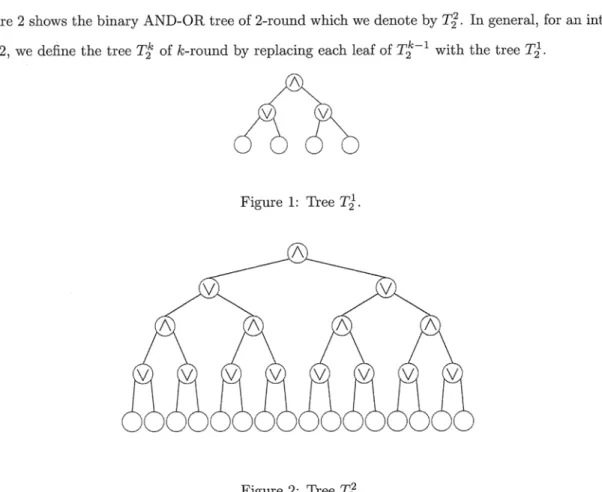
Definition 1 Figure 1 shows the binary AND-OR tree of 1-round which we denote by T. And, Figure 2 shows the binary AND-OR tree of 2-round which we denote by T. In general, for an integer k > 2, we define the tree n of k-round by replacing each leaf of with the tree T.
Figure 1: Tree Tl.
V
V A
V A
V V
V A
V
Figure 2: Tree T.
Algorithm In this paper, we restrict ourselves to a-13 pruning algorithms [1]. We will review
the concept of ct-i3 pruning algorithm later.
3
Definition 2 We assign a number to each leaf of a game tree. To the leaves in Figure 2, in the order from left to write, we assign 1, 2, 3, 4, • • • sequentially. To be more precise, the rule is described as follows: two leaves with a common parent node are assigned number 2n + 1 and 2n + 2 for some non-negative integer n; if two nodes have a common parent then for one node v of the two, it holds that the minimum number assigned to descendants of v is exactly 1 + the maximum number assigned to descendants of the other node. We denote algorithms by a permutation of leaves showing the order of scanning. For example, the algorithm that scans the leaves from left to right, which is called the algorithm of "fundamental form" in this paper, is denoted by "1234". In addition, the expression
"if(0)1234 else 1(2)43" means the following process: In the default setting , the scanning order is 1234;
in the case where the first leaf is 1 (in this case, its brother node is not scanned), the scanning order is changed to 1243, where (2) denotes that the leaf of number 2 is skipped. We say the algorithm
"if(0)1234 else 1(2)43" makes a flip. In general, by "flip" we mean that a given algorithm changes its scanning order depending query history.
2.2 Cost of computation
In this paper, cost, or computational complexity denotes the number of leaves queried by an algorithm during the computation deciding the root value. All other operations such as boolean operations of two values are considered to be of cost zero.
Definition 3 [2, p74] Let k be a positive integer. Let AD be a deterministic algorithm and w an assignment to the leaves of tree T. By C(AD, w), we denote the number of leaves queried by AD during its computation on 71 under the truth assignment w. Let W be the set of all truth assignments, and d a probability distribution on W. Then pwd denotes the probability of d having value w. The average complexity C(AD, d) of AD with respect to d is defined as follows.
C (AD, d)=Epc!,C(A-D,W).
wEW
Definition 4 [2, p75] Let D be the set of all probability distributions (on W defined above), and AD (Ti') the set of all deterministic algorithms computing T. We define the distributional complexity P(71) as follows.
P(n) = max min C (AD , d).
dED ADEAD(n)
If a distribution 8 E D achieves P(T2 ), it is called the eigen-distribution.
min C(AD, S) = P(T~
AD E.AD (Tz )
2.3 Alpha-beta pruning algorithm
The a-/3 pruning algorithm is a special type of depth-first algorithm, and is known as efficient one among many game tree algorithms. We show two examples.
Example 1 We consider the deterministic algorithm 1234, that is, the algorithm searches leaves from left to right. We assume that the truth assignment to the leaves is as shown in Figure 3. The algorithm reads 0 first. And it moves to the right leaf and reads 0. As a result, the node V above them has value 0. Then, regardless of the values of two remaining leaves, we know that the root (A) has value 0.
Hence, the computation ends. Thus, we may skip scanning the remaining two nodes. Such a skipping is called a-cut. The number of scanned leaves is two. Hence, the cost is 2.
0
0 0 a-cut
Figure 3: An example of a-cut.
Example 2 In the same way as Example 1, we consider the deterministic algorithm 1234. Assume that the truth assignment to the leaves is as shown in Figure 4. The algorithm reads 1 first. Then, regardless of the value of the brother node, we know that the parent node V has value 1. Thus, we may skip scanning the brother node. Such a skipping is called /3-cut. In this example, the cost is 3.
5
CD 0 I 13-cut
Figure 4: An example of /3-cut.
2.4 Algorithm family
Definition 5 Let k be a positive integer. We consider deterministic algorithms for T. We define classes Alj'eix and Ak of such algorithms as follows.
Ak = {A : A is an ce-,3 pruning algorithm for n},
= {A E Ak : A has a fixed order of scanning leaves}.
By definition, it is clear that Mix C Ak . We investigate the algorithm family Ak in this paper.
2.5 Substitution of nodes and closure property
Definition 6 In this paper, substitution (of nodes) denotes the operation of exchanging two nodes (internal nodes or leaves) of a common parent node. In the case of leaves then it is called substitution of leaves.
Definition 7 For each /3 C Ak, let cl(0) be the transitive closure of /3 with respect to substitution.
More precisely, as follows.
{A : 3B E /3 : a finite product of substitutions such that A = crB}.
In the case of 0=c1(13), we say "/3 has the closure property" or ",(3 is closed under the substitution
of leaves and nodes".
2.6 Reverse assigning technique
Liu and Tanaka introduce the concept of 1-set and 0-set as a set of assignments with root values 1 and 0 respectively. Roughly speaking, it is a set of assignments which requires much cost. The method forming these set is called Reverse Assigning Technique, and is abbreviated to RAT.
Methodology 8 (Reverse Assigning Technique: RAT) [2, p75-76,Methodology 6] The 1-set (0-set, respectively) of a tree T2 is defined as follows.
(1) Assign a 1 (respectively, 0) to the root of tree II.
(2) From the root to the leaves, assign 0 or 1 to each child nodes of every internal node as follows:
• for the nodes labeled A with value 1, assign is to both its child nodes;
• for the nodes labeled V with value 0, assign Os to both its child nodes;
• for the nodes labeled A with value 0, assign at random 0 to one child node and 1 to the other;
• for the nodes labeled V with value 1, assign at random 1 to one child node and 0 to the other.
(3) Form the 1-set (0-set, respectively) by collecting all the possible assignments.
We give examples of construction of 1-set and 0-set by RAT.
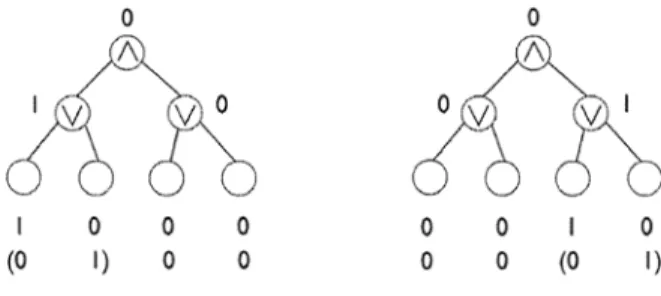
Example 3 We form an 1-set for a tree T2 (see Figure 5). First, we assign a 1 to the root of the tree T1. Since the root A is labeled with value 1, we assign is to all its child nodes. For each V node, since
it is labeled with 1, we assign at random 1 to one child node and 0 to the other. Hence, the 1-set for
tree 71 is {1010, 1001, 0110, 0101 } .
1 (0
0 I)
1 (0
0 I)
Figure 5 : The formation of the 1-set.
Example 4 We form a 0-set for a tree 711
T. Since the root A is labeled with value 0,
(see Figure 6). First, we assign 0 to the root of the tree we assign at random 0 to one child of the root and 0 to
7
the other. Since one of V node is labeled with 1, we assign at random a 1 one of its child node and 0 to the other child node. The other V node is labeled with 0, therefore we assign Os to both its child
nodes. Hence, the 0-set for tree 711 is {1000, 0100, 0010, 0001}.
00
A
0 v 7A 1 -/- y ..„. 0 VI
--- ,.:
C
--). (....,
1 0 0 00010
(01)0000(0 1)
Figure 6: The formation of the 0-set.
Definition 9 [2, p.76] By E'-distribution (respectively, E°-distribution), we denote the distribution on the assignments of 1-set (respectively, 0-set) such that all the deterministic algorithms have the
same complexity.
3 Previous results
In this section, we review relevant previous results.
3.1 Results of Liu and Tanaka
Assertion 1 [2, p76,Theorem 8] For any tree 71, we have, in the El-distribution(or E°-distribution), the probability of each assignment of 1-set(or 0-set) is equal to 40k11)/3 •
Assertion 2 [2, p76,Theorem 9] For any tree n, the E1-distribution is the unique eigen-distribution among all the distributions.
3.2 Results of Suzuki
This sub-section is a summary of Suzuki[3].
The case where k = 1 and root = 1
Let k = 1. Table 1 shows the values of C(AD,w) in the case where w is an element of the 1-set.
Al A2 A3 A4 A5 A6 A7 A8
1234 4312 3421 2143 3412 1243 2134 4321
W1 W2 W3 W4
1010 1001 0110 0101
2 3 3 4
3 2 4 3
3 4 2 3
4 3 3 2
2 3 3 4
3 2 4 3
3 4 2 3
4 3 3 2 Table 1 : C(AD , w) for k =1(wEthe 1-set).
Definition 10 Suppose that e is a real distribution on the 1-set such that the prob
number such that 0 < E < 1/2. By d(e), we denote the abilities of w1, w2, w3, w4 are r, 1/2-6, 1/2—c, e, respectively.
Assertion 3 [Suzuki,Theorem 1] There are uncountably many (the cardinality of the continuum) E1- distributions with respect to Alf that are not the uniform distribution on the 1-set. Hence, Assertion
1 fails (under this interpretation) with respect to A fZx .
Proof. Suppose that c is a real number such that 0 < 6 < 1/2. Let j E {1, 2, • • • , 8}. By Table 1, it holds that
3 E E
C (Ai ,d(c)) =
Therefore, for every e such that 0 < E < 1/2 {1, 2, • • • , 8}, the value C(Ai, d) is equal.
1/4.
Note that d(1/4) is the El-distribution (for
E(2 + 4) + (1/2 — e)(3 + 3) = 3, or
(3.1) E(3 + 3) + (1/2 — s)(2 + 4) = 3.
d(e) is a distribution on the 1-set such that for each qual. (e) is not the uniform distribution on the 1-set unless
Ell
ion (for k = 1) discussed in [2].
Eigen-distribution for k = 1
Assertion 2 suggests that, in the case where k = 1, d(1/4) is the unique eigen-distribution.
this part, we show that d(1/4) is not the unique eigen-distribution under the interpretation that algorithm does not change the priority of searching leaves throughout a computation.
The following Lemma 1 is implicitly shown in [2, p.76]. We explicitly prove it.
Lemma 1 Let k = 1. Suppose that d is a distribution on W.
(1) If mini<<8 C(Ai, d) > 3 then d is a distribution on the 1-set.
(2) If d is a distribution on the 1-set then min1<1<8C(Ai, d) < 3.
9
In
an
(3) "d is eigen with respect to Ab " if and only if "d is a distribution on the 1-set and mini<j<8 C(Ai,d) = 3".
Proof. For each i such that 1 <i < 16, let pi denote Prob[d =
(1) Tables 2, 3 show the values of C(AD, w) in the case where co is not an element of the 1-set.
Al A2 A3 A4 A5 A6 A7 A8
1234 4312 3421 2143 3412 1243 2134 4321
W5 W6 W7 Wg
1000 0100 0010 0001
3 4 2 2
2 2 4 3
2 2 3 4
4 3 2 2
2 2 3 4
3 4 2 2
4 3 2 2
2 2 4 3
Table 2: C(AD,w) for k = 1 (w E the 0-set).
Al A2 A3 A4 A5 A6 A7 A8
1234 4312 3421 2143 3412 1243 2134 4321
Wg W10 W11 W12
1110 1101 1011 0111
2 3 2 3
2 3 3 2
3 2 2 3
3 2 3 2
2 3 2 3
3 2 2 3
2 3 3 2
3 2 3 2
W13 W14
1100 0011
3 2
2 3
2 3
3 2
2 3
3 2
3 2
2 3
W15 W16
1111 0000
2 2
2 2
2 2
2 2
2 2
2 2
2 2
2 2
Table 3: C (A D , w) for k = 1 (w Ø the 1-set U the 0-set).
Suppose that mini<j<8 C(Ai, d) > 3. Since C(.41, d) > 3, by Tables 1, 2 and 3, we get the following;
2231 +3p2 +33 + 4234 + 3p5 + 4/36 + 2p7 + 2p8 + 2p9 + 3pio + 2pii + 3/312 + 3p13 + 2/314 + 22315 + 2/316 > 3.
Since pi +P2 + • • • +P16 = 1,
P1 +.137 +P8 +P9 + Pll +14 +P15 +P16 5_ P4 + P6.(3.2)
For each j E {2, , 8}, we get similar inequalities. By using these inequalities, it is shown that 5 < Vi < 16 pi = 0. Hence, d is a distribution on the 1-set.
(2) Suppose that d is a distribution on the 1-set. Assume for a contradiction that we have
min1<j<8 C(Ai,d) > 3.
Since C(Ai, d) = 2231+3232 +3P3 +44 > 3, we have pi < P4. Since C(A4, d) = 4Pi+3p2+3p3-1-2p4 >
3 we have pi > p4, a contradiction.
(3) Note that mini<i<8 C(Ai, d(1/4)) = 3. By this fact and the above (1) and (2), the equivalence holds.LI
The following is a remark to Assertion 2.
Assertion 4 [Suzuki,Corollary 1] (to Assertion 3 and Lemma 1) There are uncountably many (the cardinality of the continuum) eigen-distributions with respect to Alfix.
Proof. Suppose that e is a real number such that 0 < E < 1/2. Then, for each j E {1, 2, • • • , 8}, it holds that C(A3, d(e)) = 3, and hence d(e) is an eigen-distribution.
The case where k 1 and root = 0
In this part, we discuss a special case where the statement of Assertion 1 holds.
Proposition 2 Let k = 1. Suppose that d is an E°-distribution with respect to Alfix. Then, d is the uniform distribution on the 0-set. Hence, d is the E°-distribution of [s].
Proof. For each i e {5, 6, 7, 8}, let pi = Prob[d = wi]. Then we have 2p5 2/36 + 2/37 + 2/38 = 1.
Hence, we get the following;
C (Ai , d) =- E Cleaf=r (Ai,d) =-
r=-0
2 + p5 + 2P6
2 + 2p7 +p8
2 + P7 + 2Ps
2 + 2p5 + P6
if j E {1,6}, if j E {2,8}, if j E {3,5}, if j E {4,7}.
(3.3)
Since d is an E°-distribution, the right-hand side of (3.3) does not depend on i. Thus it holds that P5 - P6 =- P7 = P8 = 1/4.0
Now, the following assertion in [2] is justified.
Proposition 3 [2, p.76] Let k = 1. Let E° denote the (unique) E°-distribution for k = 1. If a distribution d on W is such that Prob[root = 0] = 1 and that d is not E°, then it holds that
min C (AD, d) < min C (AD, E°) = 2.75.(3.4)
ADEADADEAD
11
Proof. (sketch) The 0 value of root is achieved in the case where i E (the 0-set) U {con, w14, w16} •
By using Tables 2 and 3, we can show the proposition.^
Eigen-distribution for k > 2
Assertion 4 holds without assumption of k = 1.
Assertion5 [Suzuki,Theorem 2] Consider the case where an algorithm does not change the priority of searching leaves throughout a computation. Under this interpretation, for every positive integer k, there are uncountably many (the cardinality of the continuum) eigen-distributions.
Proof. (sketch) By means of Lemma 1 and Proposition 3, we can show the following (*).
(*) Suppose n is a positive integer. Then, for every E1-distribution d1 for k = 1, there is an eigen-distribution do for k = n such that the first round (the subtree consisting of the root, its child nodes and their child nodes) of dm is d1.
By Assertion 4, the current theorem holds.^
4 Algorithm family closed under substitution
We investigate algorithm families closed under substitution. In this section, we discuss the case where an algorithm family contains the fundamental form. The case where an algorithm family does not include the fundamental form but has closure property will be discussed in §5.The case where an algorithm family does not have closure property will be discussed in §6.
First, we investigate Afix and Ak (k > 1). In the case of k = 1, we get the following.
A f ix = { 1234, 4312, 3421, 2143, 3412, 1243, 2134, 4321}
= cl({1234})
Al = {1234, 4312, 3421, 2143, 3412, 1243, 2134, 4321,
if (0) 1234 elsel(2)43, i f (0) 4312 else4(3)21, if (0) 3421 else3(4)12, if (0) 2143 else2(1)34, if (0) 3412 else3(4)21, i f (0) 1243 elsel(2)34, i f (0) 2134 else2(1)43, i f (0) 4321 else4(3)12}
= cl({1234, if (0)1234 elsel(2)43})
= cl({1234}) U cl({if (0)1234 elsel(2)43}) (disjoint union)
Thus, in the case of k = 1, minimal algorithm families of closure property are A f ix and its
complement only, and Al is a disjoint union of the two. Hence, the following holds for k = 1.
Theorem 4 Suppose that /3 is a subset of Al that includes the fundamental form (in other words, 1234 E ,8 C ), and suppose that /3 is closed under substitution. Then, /3 is either Alfix or Al.
We ask whether the same holds for the case of k > 2.
Hypothesis 5 Suppose that is a subset of Ak that contains the fundamental form, and suppose that 13 is closed under substitution. Then, 15 is either Alf. ix or Ak .
The case of k = 2 has huge number of algorithms. As a preliminary work, we consider the case
where two trees of the form T1. are connected by a V node (see Figure 7). We denote the resulting tree by TP5.
0
(A (A
Figure 7 : Tree Tj-.5
In the case of k = 1, the number of leaves is just 4. And, we can have "the flip of scanning order"
at most once, which happens only after 0-cut. However, in the case of k = 1.5, the number of leaves is 8, and "the flip" has three possible patterns; one is after a-cut, and the others are after 0-cut. Thus, we have more complicated algorithms than the case of k = 1. Now, we partition (Aifi5x and) Al-.5 into disjoint components, where each component corresponds to a pattern of occurrences of a-cut and /3-cut.
AL5
= cl(A(12345678
=-