A Study on the Effect of Feature Selection against Categorical and Numerical Features in Fixed-length DNA Sequence Classification

A Study on the Effect of Feature Selection against Categorical and Numerical Features in Fixed‑length DNA Sequence Classification

著者 ファン ダウ

著者別表示 Phan Dau journal or

publication title

博士論文本文Full 学位授与番号 13301甲第4626号

学位名 博士（工学）

学位授与年月日 2017‑09‑26

URL http://hdl.handle.net/2297/00054255

doi: 10.4236/jbise.2017.108030

Creative Commons : 表示 ‑ 非営利 ‑ 改変禁止 http://creativecommons.org/licenses/by‑nc‑nd/3.0/deed.ja

Dissertation

A Study on the Effect of Feature Selection against Categorical and Numerical Features in Fixed-length DNA Sequence Classification

Graduate School of

Natural Science & Technology Kanazawa University

Division of Electrical Engineering and Computer Science

Student ID No.: 1424042019 Name: Phan Dau

Chief advisor: Professor Kenji Satou

Date of Submission: June 30 ^th , 2017

i

Abstract

DNA sequence classification can be defined as a process that classifies unknown DNA sequences into labelled classes. DNA sequence classification methods are categorized in three-fold. The key steps in the first category, distance- based methods, include defining distance functions to weigh the similarity between two DNA sequences, then applying present classification algorithms like k-nearest neighbor algorithm. For second group, feature-based methods, DNA sequences, firstly, are encoded into numerical feature vectors, then conventional algorithms like support vector machines are applied to classify DNA sequences. The last group are model-based methods. They are related to applying hidden Markov model or employing statistical models to address the problem of DNA sequence classification.

In order to solve this problem, there were several studies that used numerical features such as k-mer to classify DNA sequences. There were also researches using categorical features. However, the combination of numerical features and categorical features have not been studied. K-mer frequency, for example, is well-known numerical feature but position-independent. Sequences with different lengths are encoded into the same size of feature vectors, but positional information is ignored.

In contrast, categorical feature such as subsequence at a position are position-specific.

It provides positional information, but it loses quantitative information. Therefore, it can be expected that the combination of quantitative and positional information could help improve the classification performance. Moreover, it is not clear that whether or not a feature selection algorithm could be effective on the union of the numerical and categorical features of DNA sequences. By utilizing the combination of numerical features like k-mers and categorical features like subsequences starting at a specific position of given DNA sequence, in this research, we developed a simple but efficient model for improving the performance of fixed-length DNA sequence classification.

The proposed model was evaluated on six benchmark datasets. Promoter and

Splice dataset were downloaded from UCI machine learning repository. Human,

worm and fly datasets are benchmark datasets which were developed by Guo et al. in

2014, and yeast dataset is the benchmark dataset developed by Chen et al. in 2015.

ii

The performance results of our model were comparable or better than those of active algorithms. The most noticeable thing is that our method reached the accuracy of 100% on two datasets: Promoter and yeast datasets. What more is that by performing feature selection on numerical and categorical features, we could also discover which group of features are more effective on which dataset.

Keywords: Sequence classification, Numerical and categorical features, Feature

selection

iii

Acknowledgements

After three years studying at Kanazawa University, this thesis is the best award for me. I believe that the completion of this work would have been immeasurably more difficult if without the help and support from the kind people. Therefore, I wish to take this opportunity to gratefully acknowledge the assistance and contribution of everyone who made my work accomplish fully.

First of all, I am deeply thankful to my supervisor, Professor Kanji Satou for his enthusiasm, encouragement and support. I thank him for providing me a chance to do research at the Bioinformatics Laboratory, Kanazawa University. His advice on both research and daily life have been precious for me.

I am earnestly grateful to all committee members, Professor Kenji Satou, Professor Takeshi Fukuma, Associate Professor Yoichi Yamada, Associate Professor Hidetaka Nambo, and Associate Professor Makiko Kakikawa for reading my thesis and giving brilliant comments and suggestions.

Thanks are also due to the Board of Kien Giang 120 Project under Mekong 1000 Project for offering me the scholarship. This scholarship has played a key role in achieving my educational dreams.

I would like to thank Kanazawa University for providing me a chance to take the PhD course here. My great thanks are extended to the staff of Kanazawa University who are friendly, polite and enthusiastic. It is strongly believed that my studying here would be more difficult if I did not get assistance and help from them.

I deeply thank to all colleagues at Kien Giang Teacher’s Training College, especially to the Managing Board of College who allowed me take the PhD course. Moreover, their encouragement and help enabled me to overcome difficulties and challenges.

My sincere thanks also goes to Vietnamese students’ Union at Kanazawa University

(Vietkindai) for what the Union has done for us. It makes me feel Kanazawa land as

my second home where there are so many friends who I can share my feelings when

I feel sad or happy. I would like to show my deep gratitude to two Japanese uncles,

iv

Yukio Abe and Mi Tetuo for their support and contribution to the success of the Union.

My deep thanks also go to my friends at the Bioinformatics Laboratory, Kanazawa University for wonderful moments we have worked together. I wish to acknowledge the help provided by all my labmates, Vu Anh, Sergey, Duc Luu, Ngoc Giang, Rosi, Bahriddin, Reza, Bedy and Mera, who shared their expertise and experiences with me, and provided me valuable feedbacks and suggestions.

Last but not the least, I owe my deepest gratitude to my parents, parents-in-law, brothers, sisters, especially my wife and my daughter. They have always stood by me in all situations. Most importantly, I am forever indebted to my wife and my daughter for their love, understanding and encouragement. They have been waiting my return with much patience for three years to become a complete family.

Thank you so much!

v

Table of Contents

Chapter 1 : Introduction ... 1

1.1. Research context ... 2

1.2. Objectives ... 4

1.3. Contributions ... 8

1.4. Organization... 9

Chapter 2 : Related Works ... 10

2.1. Splice site prediction review ... 11

2.2. Promoter prediction review ... 13

2.3. Nucleosome positioning prediction review ... 15

2.4. Learning Machine Algorithms ... 16

2.4.1. Artificial Neural Networks (ANNs) ... 16

2.4.2. Convolutional Neural Networks (CNNs) ... 18

2.4.3. Support Vector Machines (SVMs) ... 19

2.4.4. Random Forests ... 20

2.4.5. k-Nearest Neighbor Algorithms ... 22

2.5. Feature Selection ... 23

2.5.1. Filter Methods ... 24

2.5.2. Wrapper Methods ... 25

2.5.3. Embedded Methods ... 26

2.6. Classification Evaluation ... 26

2.6.1. Classification Evaluation Metrics ... 26

2.6.2. Cross-Validation ... 28

2.6.3. Leave-one-out cross-validation (LOOCV) ... 29

2.6.4. Bootstrap ... 30

Chapter 3 : Materials and Methods ... 32

3.1. Datasets ... 33

3.1.1. Promoter and Splice datasets ... 33

3.1.2. Nucleosome benchmark datasets ... 34

3.2. Features ... 35

vi

3.3. Algorithm ... 37

3.4. Feature Selection ... 39

Chapter 4 : Experimental Results and Discussion ... 41

4.1. Feature Ranking by Random Forest ... 42

4.2. Prediction Accuracy of Feature Subsets along Ranking ... 44

4.3. Prediction accuracy of neighbors around the best feature subset ... 45

4.4. Evaluation ... 47

4.4.1. Evaluation Metrics ... 47

4.4.2. Performance Evaluation of the Method ... 47

4.5. Comparison with other methods ... 47

4.5.1. Summary of existing models ... 47

4.5.2. Comparison on Promoter and Splice datasets ... 49

4.5.3. Comparison on nucleosome positioning datasets... 51

4.6. Discussion and Conclusion ... 53

Chapter 5 : Summary and Future Research ... 55

5.1. Dissertation summary ... 56

5.2. Future Research ... 57

Bibliography ... 60

vii

List of Figures

Figure 1.1. The number of sequences in GenBank and WGS ... 2

Figure 1.2. The process of gene expression. (Source [11]). ... 5

Figure 1.3. Promoter position in DNA sequence ... 6

Figure 1.4. Two types of splice junctions in a DNA sequence. ... 6

Figure 1.5. The structure of nucleosome. (Source [13]) ... 7

Figure 2.1. The EMSVM model proposed by Maleki et al. [45] ... 14

Figure 2.2. The general model of an ANN. ... 17

Figure 2.3. The operation of a neuron. ... 18

Figure 2.4. LeNet5 Architecture. (Source [59]) ... 18

Figure 2.5. A simple structure of CNN for recognizing image. ... 19

Figure 2.6. An example of random forest. ... 21

Figure 2.7. Flowchart of KNN algorithm. ... 22

Figure 2.8. The general process of dimensionality reduction. ... 24

Figure 2.9. A general framework for filter methods ... 25

Figure 2.10. A general framework for wrapper methods ... 26

Figure 2.11. A general framework for embedded methods ... 26

Figure 2.12. A procedure of 10-fold cross-validation. ... 29

Figure 2.13. A procedure of leave-one out cross-validation ... 30

Figure 3.1. Splice-junction gene sequence ... 34

Figure 3.2. Promoter sequence in DNA sequence. ... 34

Figure 3.3. The overview of the basic entities forming chromatin. (Source [79])... 35

Figure 3.4. The flowchart of the proposed algorithm. ... 38

Figure 3.5. Step 1 of the feature selection algorithm. ... 40

Figure 4.1. MeanDecreaseAccuracy along feature ranking from top 1~ 60. ... 42

Figure 4.2. MeanDecreaseAccuracy of features in 2CAT vector on (a) Splice and (b) Promoter datasets. ... 44

Figure 4.3. The percentage of feature groups in the best feature subsets. ... 46

Figure 4.4. The structure of convolutional neural network. (source [76]) ... 48

Figure 4.5. Our method and reported methods in ROC space. ... 51

viii

List of Tables

Table 2.1. Several popular models for detecting splice sites from 1997 to 2003. ... 11

Table 2.2. Confusion matrix for a binary classifier ... 27

Table 3.1. Description of datasets ... 33

Table 4.1. List of important features. ... 43

Table 4.2. Prediction accuracies obtained by using either the whole set of features and the best feature subset in step 1. ... 45

Table 4.3. Prediction accuracies in step 2 compared with those in step 1. ... 45

Table 4.4. Accuracies of the proposed model compared to those in [76]. ... 49

Table 4.5. Comparison our method with other reported methods. ... 50

Table 4.6. Performance comparison of our model and previous models. ... 52

1

Chapter 1 : Introduction

We begin in section 1.1 by introducing a research context of the thesis and

various types of sequence classification methods. These include distance-based

methods, feature-based methods and model-based classification. Objectives of the

thesis are mentioned in section 1.2. We describe the contributions of the thesis in

section 1.3. Lastly, in section 1.4 we show the organization of the thesis.

2

1.1. Research context

In recent years, biological data have been generated at a tremendous rate.

According to [1], the number of DNA sequences contained in GenBank repository increased dramatically from 116,461,672 to 181,336,445 between February 2010 and February 2015 (as shown in Figure 1.1). The sequences in UniProt doubled during the period of just one year, from 40.4 (June 2013) to 80.7 (August 2014) million [2].

Analysis and interpretation of these data are two of the most crucial tasks in bioinformatics, and classification and prediction methods are key techniques to address such tasks.

Figure 1.1. The number of sequences in GenBank and WGS

As summarized by Xing et al. [3], there were three main groups of the DNA

sequence classification approaches. The first class includes methods that firstly define

distance functions to compute the similarity between two sequences. After that, some

of the current learning algorithms like k-nearest neighbor are applied. The second

category is feature-based methods. Before employing conventional algorithms such

as decision trees and artificial neural networks to classify DNA sequences, these

sequences need to be encoded into feature vectors. So as to enhance the performance,

feature selection plays a key role in this type of methods. The last type is a group of

methods like Markov Models and statistical algorithms used to perform sequence

classification.

3

With regard to the first category, in the research of by Borozan et al. [4] in 2015, they exploited the complementarity of alignment-free and alignment-based similarity to classify biological sequences. They used five different sequence similarity measures: three out of five measures were alignment-free and the other two belonged to the second category of measures, which revealed that their model outperformed previous models. In 2014, Chen et al. [5] also tackled the problem of categorical data in a typical distance-based manner. They defined four weighted functions for categorical features, two of them named as simple matching coefficient measures with global weights (WSMC

) and the other two named as simple matching coefficient measures with local weights (WSMC

), then applied these functions to formulate new nearest neighbor classification algorithms. The classifiers were evaluated by using real datasets and biological datasets. The results showed that their proposed classifiers outperformed the traditional methods.

Moving to the second class, the application of feature selection technique and feature-based method to classify protein sequence data was carried out by Iqbal et al [6] in 2014. The experimental results of their research showed that their model significantly improved in terms of accuracy, sensitivity, specificity, F-measure, and other performance measure metrics. In the study of Weitschek et al. [7] in 2015, they used the combination of alignment-free approaches and rule-based classifiers so as to classify biological sequences. At first, the biological sequences were converted into numerical feature vectors with alignment-free techniques, then rule-based classifiers were applied in order to assign them to their taxa.

The study about classifying occupancy, acetylation, and methylation of

nucleosomes was carried out by Pham et al. [8]. Their method was also a kind of

feature-based classification, which converted sequences into numerical feature

vectors, then applied a conventional classification method. They adopted SVM with

RBF kernel, and feature vectors were k-mer based vectors with a variety of window

sizes (k =3, 4, 5, 6, etc.). Using ten datasets collected by Pokholok et al. [9], they

gained a high prediction accuracy. To get better performance results, a technique

termed feature selection was used by Higashihara et al. [10] to solve this problem. In

this research, the importance of features was first measured by MeanDecreaseGini

4

value computed through training and prediction by random forest, then features were ranked as the order from the most to least importance. Exploiting feature selection along feature ranking, they achieved slight improvements in prediction accuracy.

What is more, by searching neighbors of the best feature subset, accuracy of prediction improved further.

Although the active researches on sequence classification above, numerical and categorical features were separately studied until now. Since the numerical features like k-mer are typically position-independent and categorical features like nucleotide at a position are position-specific, we can expect that these two types of features could contribute to the classification performance in a complementary manner. In addition, it is still unclear how effective a feature selection algorithm is against the union of numerical and categorical features of sequence. In this study, we propose an effective framework for improving fixed-length DNA sequence classification by using the combination of categorical features (i.e. subsequence at a position like “A”, “AG”, etc.) and numerical features (i.e. k-mer frequency). By conducting feature selection on this mixture of features, we could also find which type of features are more effective in each dataset.

1.2. Objectives

The major target of our thesis is that we develop an effective model to address the problem for classifying fixed-length DNA sequences. The specific objectives are as follows.

Applying a proposed model to classify promoter sequences

In genetics, gene expression is the series of biological actions which is related to using DNA of the gene to synthesize the functional product. These functional products are often proteins which have important roles in organisms, including catalyzing reactions, transporting molecules like oxygen, keeping organisms healthy and transmitting messages. The process of gene expression has two key stages:

transcription and translation. The first stage of gene expression is transcription, which

engages in copying information from a gene to produce an RNA molecule (especially

5

mRNA). This step is performed by enzymes called RNA polymerases, which use a DNA strand as a template to form an RNA. Translation is the second stage of gene expression. It is the process of translating the chain of a messenger RNA molecule to a chain of amino acids, polypeptide. The polypeptide then folds into an active proteins and fulfils its functions in the cell. The diagram in Figure 1.2 shows a process of gene expression in a eukaryote.

Figure 1.2. The process of gene expression. (Source [11]).

A promoter is the part of DNA sequence which are sited directly upstream of

the start site of transcription. Figure 1.3 shows the position of the promoter on a DNA

sequence.

6

Figure 1.3. Promoter position in DNA sequence

The most important step in the process of transcription is to determine where is a gene or where is the transcription start site. Promoter identification can help locate the position of gene and then analyze the process of gene expression. Therefore, promoter prediction and promoter classification are two considering problems in the field of bioinformatics, and classifying promoter sequences is the first objective of our research.

Applying a proposed model to classify splice sequences

During transcription process, the pre-mRNA is stranscribed from a DNA of gene. This pre-mRNA must be processed in order to become a mature messenger RNA (mRNA) that can be translate into a protein. The step of processing the pre- mRNA to become mature mRNA is called as RNA splicing, and it is carried out by spliceosome. Since pre-mRNAs include introns and exons, hence introns must be removed by the process of splicing to form mature mRNAs. After the process of RNA splicing, mature mRNAs are translated into proteins. Two types of splice junctions are exon-intron (EI) and intron-exon (IE) junctions. The first one is called a donor site that usually contains dinucleotides GT. However, the later is named as an acceptor site which often includes dinucleotides AG [12]. Figure 1.4 illustrates the positions of them in the DNA sequence.

Figure 1.4. Two types of splice junctions in a DNA sequence.

RNA – coding region Promoter

Downstream Upstream

DNA 5’ 3’

Terminator

Exon Exon

AG GT

Intron

IE EI

DNA sequence

7

In eukaryotes, the first important works for predicting gene is to predict splice junctions. Therefore, developing an effective model for accurately predicting splice junctions is an attractive work, and it is also the second goal of our research.

Applying a proposed model to classify nucleosomal sequences

In eukaryotes, one of the fundamental parts forming chromatin includes nucleosome. Every nucleosome is composed of a segment of roughly 147 base pairs (bp) which is called a nucleosome core particle being covered stiffly around a histone octamer [13]. In order to form the histone octamer, eight histone proteins are used.

They include two H2As, two H2Bs, two H3s and two H4s as shown in Figure 1.5.

Two nucleosome core particles are connected each other by a linker DNA sequence.

Several researches indicated that nucleosome core particle played crucial roles in biological processes like DNA replication and DNA repair [14], [15], [16], [17], [18].

Therefore, predicting nucleosome positioning sequences (or nucleosomal sequences) is fundamentally important in bioinformatics. This problem is also thirdly addressed in our research.

Figure 1.5. The structure of nucleosome. (Source [13])

8

1.3. Contributions

In order to classify DNA sequences, k-mer frequency, quantitative information, is commonly used since it can convert sequences with different lengths into the same size of feature vectors. However, positional information is lost in k- mer. For fixed-length sequence, it is possible to use subsequence itself as categorical value. It keeps positional information, however, quantitative information is not available. The primary goal of our dissertation is to provide a framework for classifying fixed-length DNA sequences by using both positional and quantitative information. The key contributions of present thesis can be summarized as follows.

An effective framework for improving fixed-length DNA sequence classification

There were researches that employed numerical features for DNA sequence classification. There were also studies using categorical features. However, until now there is no research that utilized the combination of categorical features and numerical feature in one model. Therefore, we developed a simple but effective model for classifying fixed-length DNA sequences by combining numerical features (quantitative information) with categorical features (positional information) in one model. Feature selection was also used so as to improve the prediction accuracy.

Applications to various biological datasets

Our framework was applied to three different types of DNA sequence datasets:

a splice junction sequence dataset, a promoter sequence dataset and four nucleosome positioning datasets. Through the performance evaluation on six datasets of fixed- length DNA sequences, our algorithm based on the above idea achieved comparable or higher results than other advanced algorithms.

Discovery of effective features

By conducting feature selection on the combination of numerical and

categorical features, we could also find which type of features are more effective in

each dataset. For Promoter and Splice datasets, categorical features, especially 2CAT

features, are more effective than other numerical features. Whereas several numerical

9

features in k-mers are so important than categorical features on nucleosome positioning datasets.

1.4. Organization

This thesis is divided into five chapters. It is organized as follows.

The current one is Chapter 1 that introduces the research context, objectives, contributions and the organization of this thesis.

Chapter 2 talks about related works. At first, we review some models for predicting promoter, splice site and nucleosome positioning sequences. Next, we highlight some well-known algorithms as well as evaluation measures that have been used in bioinformatics.

Chapter 3 describes our model in detail. We, firstly, provide a brief description of promoter, splice site and nucleosome positioning datasets. Then, we explain the general model, algorithms and evaluation measures.

Chapter 4 focuses on analyzing and discussing experimental Results. We also conduct evaluation and make further comparisons with state-of-the-art models.

Chapter 5 summarizes the thesis, highlights the achievements of our work and

suggests some future works.

10

Chapter 2 : Related Works

In this chapter, we, firstly, review models related to our research. Splice site

prediction review is done section 2.1. Then, we do promoter prediction review in

section 2.2 and nucleosome positioning prediction in the next section. Several

popular learning machine algorithms used in bioinformatics are shown in section

2.4. Next, we summarize some feature selection methods in section 2.5. Lastly, we

describe well-accepted classification evaluations in section 2.6.

11

2.1. Splice site prediction review

There are many important algorithms like Artificial neural networks, Bayesian classifiers and SVMs that have been employed to solve splice site prediction problems [19], [20], [21], [22]. Zhang et al. [23] summarized some well-known models used in prediction of splice site in the period of between 1997 and 2003 as shown Table 2.1.

Table 2.1. Several popular models for detecting splice sites from 1997 to 2003 [23].

Models References

Statistical Models:

 Logit linear algorithm Brendel and Kleffe, 1998 [24]

 Quadratic discriminant analysis Zhang and Luo, 2003 [25]

 Naïve Bayes classifier Degroeve et al., 2002 [26]

Decision trees:

 Maximal dependence decomposition Burge et al., 1997 [27]

 MDD with Markov model Pertea et al., 2001 [28]

 C 4.5 induction tree Patterson et al., 2002 [29]

Artificial neural networks:

 Percepton Weber, 2001 [30]

 Multi-layer Backpropagation Reese et al., 1997 [31]; Sonnenburg et al., 2002 [32]

SVMs:

 Linear kernels Degroeve et al., 2002 [26]

 Polynomial kernels Patterson et al., 2002 [29]

Apart from these researches, there have been a number of other studies on the prediction of splice sites as well. The study of using support vector machine for accurately predicting splice sites was introduced by Sonnenburg et al. [33] in 2007.

They applied the so-called weighted degree kernel to solve the problem of splice sites

recognition, which turned out well suitable for their work. They conducted several

experiments on splice site genomes: Arabidopsis thaliana, Danio rerio,

12

Caenorhabditis elegans, Drosophila melanogaster, and Homo sapiens. The results revealed that their model accurately identified splice sites in these genomes. Their method achieved higher performance than past methods consisting of GeneSplicer [28] and SpliceMachine [34] . The splice site prediction tool using their method was also provided.

In 2008, Baten et al. [35] introduced the research on identification of splice site by exploiting informative features and employing attribute selection. They developed the algorithm using the combination of informative features with support vector machine. They also applied a feature selection method to eliminate unimportant features. They carried out the experiments on NN269 dataset. The results showed that their method outperformed the previous methods not only prediction accuracy but also training time.

By using short sequence motifs, Meher et al. [36] in 2014 released the statistical method for predicting donor splice sites. Their approach was used to predicted these splice sites but their sequences were not converted into numerical features. The main idea of the approach exploited dinucleotide association. The method was applied to predict human genome and the performance was compared with the common methods used in researches [27] , [37], [38] . Their model achieved equal or higher accuracy than active methods. They also provided a user friendly website using this model.

Two years later, Meher et al. [39] also proposed another algorithm for solving

the above problem. In their research, splice site DNA sequences, firstly, were

converted into numerical features based on not only neighboring but also non-

neighboring dinucleotide dependencies. Then, they employed three different learning

machine algorithms to predict this type of DNA sequences. The model was tested on

H3SD, NN269 datasets, and was further evaluated on the independent dataset. By

using the independent dataset, their model obtained better accuracies compared to the

previous methods such as NNsplice, MEM, MDD, WMM, MM1, FSPLICE

(accessible at http://www.softberry.com ), GeneID [31] and ASSP [40] . An online

donor splice site prediction server (named as PreDOSS) was also provided.

13

At the same year (2016), Meher et al. [41] introduced another approach for predicting donor splice sites. Firstly, each sequence was encoded into three distinct groups of variables. They were positional, compositional and dependency variables.

The positional variables and the scores of WMM were similar. The dependency variables and the scores WAM were similar. The compositional variables were the union of 2-mer, 3-mer and 4-mer frequency. Therefore, there were 344 variables for each sequence. Then, they conducted feature selection by using F-score, and just 49 out of 344 features survived from this step. Finally, these 49 variables were used as input to support vector machine for prediction. By using human, cattle, fish, worm and NN269 datasets, results showed that their method was comparable to present methods. They also developed a website HSplice for predicting this kind of genomes.

2.2. Promoter prediction review

There have been several machine learning models for predicting biological signals like promoters that carry out the transcription process. The prediction of promoters has been attracting many researchers in [42], [43], [44], [45], [46], [47], [48], [49], [50], therefore we review some notable methods to address this problem.

In the year of 1990, Towell et al. [42] proposed a hybrid learning system named as KBANN (Knowledge-Based Artificial Neural Networks) that combined explanation- based learning and empirical learning systems. The dataset of E. coli-2 DNA sequences was also developed to help test the KBANN model. This dataset consists of 106 sequences. Half of them contains promoters known as positive samples, while another half of sequences do not contain promoters assigned as negative samples, and each of sequences has length of 57. The experimental results on this dataset showed that the KBANN outperformed the other four methods.

Czibula et al. in 2012 [43] proposed the method for predicting promoter using relational association rules named as “PCRAR”. These rules are a specific class of association rules. They can characterize the relationships between variables in a dataset. The PCRAR model did not depend on any specific biological mechanisms.

The strong point of PCRAR was that it could learn the distinctions between promoter

sequences and non-promoter sequences without using further biological information.

14

They evaluated their proposed classifier and made comparison with existing methods.

Their experimental results showed that their algorithm outperformed the existing models for identification of promoter sequences, which confirmed that their approach was a potential model for predicting promoter sequences.

The combination of expectation maximization clustering and support vector machine (EMSVM) for solving the above issue in bacterial DNA sequences was presented by Maleki el at. in 2015 [45]. There were two phases in the EMSVM algorithm. In the first stage, expectation maximization algorithm enabled to identify groups of bacterial DNA sequences that showed similar characteristics. Each of bacterial DNA sequence was clustered to different clusters with different probabilities. Then, in the second stage, the support vector machine was applied. The EMSVM model is shown in Figure 2.1.

Figure 2.1. The EMSVM model proposed by Maleki et al. [45]

To evaluate the EMSVM method, they used the four promoter datasets of E.

coli DNA sequences: 24, 32, 38 and 70. These datasets consist of sequences with length of 81 bases. The 24, 32, 38 and 70 contain 520, 309, 217 and 1907 promoter sequences (positive samples), respectively. Each of these datasets also

Sequence1 ATCGTCDAGGT

Sequence2 GTTACAATGCA

… ……..

Expectation Maximization Clustering

Cluster1 Cluster2 …

Sequence1 0.11 0.09 …

Sequence2 0.08 0.12

… … … ..

Support Vector Machine Classifier

15

includes 2000 non-promoter sequences (negative samples). Moreover, they evaluated their proposed algorithm on the E. coli-2 dataset as well. Four distinct evaluation metrics were used to evaluated this method. Their results demonstrated that EMSVM achieved higher performance than other methods.

Lin et al. [44] proposed another model, named as “iPro54-PseKNC”, in 2014.

In this model, firstly, promoter and non-promoter sequences were encoded into feature vectors, named as “pseudo k-tuple nucleotide composition”. Next, these feature vectors were used as the inputs to support vector machine. To evaluate iPro54- PseKNC predictor, they used sigma 54 dataset and four evaluation metrics: Accuracy, specificity, sensitivity and Matthews correlation coefficient. The web server named iPro54-PseKNC was also developed.

2.3. Nucleosome positioning prediction review

A number of studies have been attempted to developed models for predicting nucleosome positioning. Herein, we summarized some methods for nucleosome positioning released recently. In 2010, Yi et al. [51] introduced a model for solving this problem by using transcription factor binding sites (TFBSs) and the nearest neighbor algorithm. In this research, by using an online server of MatInspector [52], both nucleosome-forming and nucleosome-inhibiting sequences were converted into feature vectors with the length of 35 transcription factor binding sites (TFBSs). Next, they conducted feature selections by using two distinct approaches to reduce the size of feature vectors. Nine important features (families of TFBSs) were identified, then nearest neighbor algorithm was applied to predict around 53000 nucleosome-forming and about 50000 nucleosome-inhibiting sequences in yeast genome. With the jackknife cross-validation test, the prediction accuracy reached 87.4%.

In the research of Guo et al. [13] in 2014, they proposed a predictor named as

‘iNuc-PseKNC’ that was applied to predict nucleosomal sequences in human, worm

and fly genomes. First of all, DNA sequences in datasets were transformed to feature

vectors by employing a novel formula named as “pseudo k-tuple nucleotide

composition”. Then, support vector machine algorithm was applied to classify DNA

sequences into 2 classes: nucleosome-forming and nucleosome-inhibiting classes.

16

Jackknife test was also conducted to assess their method performance. They released an online server for predicting these three kinds of genomes as well.

In 2016, Tahir and Hayat [53] introduced a predictor (called “iNuc-STNC”) for prediction of nucleosome positioning in three above genomes. Nucleosome sequences were encoded into three different groups of features like 2-mer, 3-mer and split 3-mer composition. By applying support vector machine, the performance results on three benchmark datasets (human, worm and yeast) demonstrated that their model was effective on identifying nucleosome positioning sequences.

To address this problem, in early 2017 Awazu [54] developed two novel nucleosome positioning prediction models based on the combination of three kinds of features with different segment length scales. Models employed linear regression algorithm to predict nucleosomal sequences, and they were named as 3LS (three length scales) and TNS (Tri-nucleosome sequence). 3LS model achieved better results than the past methods on Homo sapiens and Drosophila melanogaster genomes, and TNS reached 100% accuracy on Saccharomyces cerevisiae genome.

2.4. Learning Machine Algorithms

There are many well-know learning algorithms used in bioinformatics.

However, in this thesis, we just concentrate on several algorithms that are commonly used in splice site, promoter and nucleosome positioning prediction.

2.4.1. Artificial Neural Networks (ANNs)

ANNs are computational methods which were firstly invented in 1943 by

Warren McCulloch and Walter Pitts. The key idea of an artificial neural network is

simulating the human brain [55]. In the years of 1950s, with the development of the

perceptron network and associated learning rule by Frank Rosenblatt, ANNs were

firstly applied in the field of pattern recognition. However, now ANNs have been

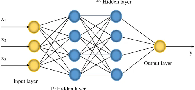
applied in various disciplines. In general, an artificial neural network contains three

parts, known as layers. An example of an artificial neural network is shown in Figure

2.2.

17

The input layer has responsibility for collecting information data, signals, features from the outside environment.

The hidden layers are made of neurons which are in charge of the performance of the internal processing from a network.

The output layer includes neurons which are responsible for yielding and presenting the final network outputs.

Figure 2.2. The general model of an ANN.

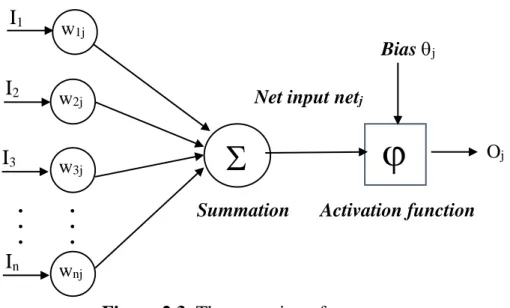
ANNs are constructed from layers of connected neurons. Therefore, each neuron at hidden layers and output layer receives inputs from neurons at the preceding layer and passes the output to neurons at the succeeding layer. These neurons operate in Figure 2.3 [56], [57].

I

, I

, …, I

are the inputs for the neurons.

w

, w

, …, w

are the weights.

Summation = I

.w

+ I

.w

+ … + I

. w

Input layer x

x

x

y

1

Hidden layer

2rd

Hidden layer

Output layer

18

Figure 2.3. The operation of a neuron.

2.4.2. Convolutional Neural Networks (CNNs)

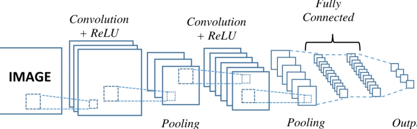
CNNs are one specific class of Artificial Neural Networks. They have been successfully adopted in different fields of researches like image recognition. These days, convolutional neural networks play crucial roles in the field of machine learning.

The early convolutional neural network was the LeNet Architecture (LeNet5) developed by Yamm LeCun in 1990s [58]. Figure 2.4 is the architecture of LeNet5 for recognizing characters like reading zip codes and digits, and so forth.

Figure 2.4. LeNet5 Architecture. (Source [59])

Figure 2.5 is the structure of a CNN that has the similar architecture of the LeNet5 [58]. However, this model was used for classifying images. There are four leading operations in the convolutional neural network (shown in Figure 2.5).



w

w

w

w

 ^O

. . .

. . .

I

I

I

I

Summation

Net input net

Bias 

Activation function

19

Figure 2.5. A simple structure of CNN for recognizing image.

From the first convolutional neural networks, LeNet, was invented in early 1990s. Some other convolutional neural networks have been evolved, and they are listed as follows [58].

In 2012, AlexNet was presented by Alex Kirzhevsky et al. This convolutional neural network had more neurons and layers than the LeNet. It was a winner in ImageNet Large Scale Visual Recognition Challenge (ILSVRC) at that time.

In 2013, the winner in ILSVRC was ZF Net (stand for Zeiler and Fergus Net) which was developed by Matthew Zeiler and Rob Fergus.

In 2014, GoogLeNet was a winner in ILSVRC. This convolutional neural network was introduced by Szegedy et al. from Google.

In 2015, The winner in ILSVRC was Residual Network (ResNets) that was developed by Kaiming He et al.

Recently, August 2016, Huang et al. introduced the Densely Connected Convolutional Network (DenseNet). The DenseNet outperformed previous network architectures on five object recognition benchmark datasets.

2.4.3. Support Vector Machines (SVMs)

In machine learning, SVMs have been used for classification as well as regression. They can conduct not only on linear data but also on nonlinear data.

Support vector machines were invented in mid – 1960s by Vapnik et al. However, until 1992, the journal article about support vector machines was firstly published,

IMAGE

Convolution + ReLU

Convolution + ReLU

Pooling Pooling

Fully Connected

Output

20

and the authors of the paper were Vapnik and his colleagues [60]. The overview of its algorithm works as following. Support vector machine, firstly, uses a special mapping to convert the lower dimension data into a higher dimension data. Then, it finds a linear optimal hyperplane that divides tuples of one group from another group.

Support vector machine searches for this hyperplane based on support vectors (the samples that are essential to detect classes) and margins. Support vector machines have been applied to various areas, consisting of digit recognition [61], image recognition [62], text classification [63], sequence classifications [64] and so forth.

Some main advantages and disadvantages of support vector machine can be summarized as follows [65]:

Advantages:

- Support vector machine can work effectively in high dimensional spaces.

- Support vector machine performs much better when there is a clear margin of separation.

- Support vector machine is memory saving algorithm since it uses a subgroup of training instances called support vectors to formulate a decision function.

Only these support vectors must be stored in memory in order to make decisions.

Disadvantages:

- Support vector machine does not work very well on datasets with more noise.

- Support vector machine does not directly yield probabilistic estimates for group membership.

2.4.4. Random Forests

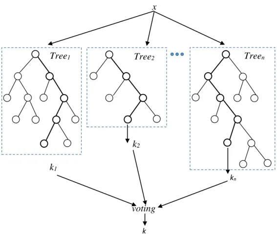
Random Forests were invented by Breiman et al. in 2001 [66]. They are

ensemble learning methods that can be used for classification as well as regression

[60], [67]. At the training phase, random forests build a lot of decision tree classifiers

so that the collection of these individual classifiers forms random forests. During

classification, output class of random forests is the voting of the output classes

produced by individual classifiers [60]. Figure 2.6 is an example of random forest.

21

Figure 2.6. An example of random forest.

Random forests are the popular algorithms for not only classification but also regression. However, random forests have been more widely used for classification models than for regression models. Some features of Random Forests can be listed as following [68].

- In the terms of accuracy, it is not the best one among latest algorithms.

However, it can work efficiently on the big datasets. Moreover, random forest has ability to handle data with a high dimension, thousands of input features.

- Random forest has a good algorithm for estimating missing data so that it can work well on the data with a large proportion of missing.

- When random forest has been generated, it can be saved for later use.

- Random forest can measure the importance of features in the classification.

- Random forest provides an effective algorithm for detection of feature interactions.

Tree

Tree

x

k

k

k

voting

k

Tree

22

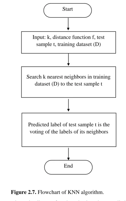
2.4.5. k-Nearest Neighbor Algorithms

In the early 1950s, the k-nearest neighbor algorithm was introduced but it was not popular. Until the 1960s, the k-nearest neighbor algorithm was commonly used since there was a significant increase in computing power [60]. The general flowchart of k-nearest neighbor algorithm (KNN) is illustrated in Figure 2.7.

Figure 2.7. Flowchart of KNN algorithm.

There are several popular distance functions that have been applied to compute the distance of two points pp and qq in a feature space. Given pp = (pp

, pp

, …, pp

) and qq = (qq

, qq

, …, qq

) are two points in an n-dimension feature space.

Start

Input: k, distance function f, test sample t, training dataset (D)

Search k nearest neighbors in training dataset (D) to the test sample t

Predicted label of test sample t is the voting of the labels of its neighbors

End

23

Euclidean distance:

𝑑(𝑝𝑝, 𝑞𝑞) = √∑ ^𝑛 _𝑖=1 (𝑝𝑝 _𝑖 − 𝑞𝑞 _𝑖 ) ²

Squared Euclidean distance:

𝑑(𝑝𝑝, 𝑞𝑞) = ∑ ^𝑛 _𝑖=1 (𝑝𝑝 _𝑖 − 𝑞𝑞 _𝑖 ) ²

Manhattan distance:

𝑑(𝑝𝑝, 𝑞𝑞) = ∑ ^𝑛 _𝑖=1 |𝑝𝑝 _𝑖 − 𝑞𝑞 _𝑖 |

Minkowski Distance:

𝑑(𝑝𝑝, 𝑞𝑞) = (∑(𝑝𝑝 _𝑖 − 𝑞𝑞 _𝑖 ) ^𝜆

𝑛

𝑖=1

) ^{1 𝜆}

Cosine similarity:

cos(𝑝𝑝, 𝑞𝑞) = ^{∑ 𝑝𝑝 𝑖 . 𝑞𝑞 𝑖}

𝑛 𝑖=1

√∑ ^𝑛 _𝑖=1 𝑝𝑝 _𝑖 ² √∑ ^𝑛 _𝑖=1 𝑞𝑞 _𝑖 ²

2.5. Feature Selection

In recent decades, dataset size, the number of instances as well as of attributes, have been exploding at the great considering levels. Consequently, storing and processing these data have been becoming more challenging, and machine learning methods also have difficulties in coping with the big data. In order to implement machine learning methods more effectively, pre-processing of the data is needed.

Dimensionality reduction is one of the most popular and important techniques to

remove noisy and redundant features, and has become an absolutely essential step

machine learning process. The general model for dimensionality reduction is shown

in Figure 2.8 [69]. This step enables to speed up data mining algorithms, improve

prediction accuracy. The first class of dimensionality reduction is feature extraction,

and the second one is feature selection.

24

Figure 2.8. The general process of dimensionality reduction.

Feature extraction can be defined as the process of projecting the input data with a higher dimensionality into a new space with lower dimensionality.

Feature selection, however, can be defined as the process of detecting relevant features and eliminating irrelevant, redundant features. The main objectives of feature selection are threefold [70], [71], [72]: reducing computational time, improving prediction performance and understanding data deeply. There are three major categories of feature selection methods.

2.5.1. Filter Methods

Filter feature selection methods are mainly based on a number of statistical measures such as Pearson Correlation and Mutual Information, to assign different features with different scores [73]. The features with the best scores are used in building the model while others are not used for analysis. These methods are not dependent on any particular classifiers, as shown in Figure 2.9.

High Dimensional Data

Low Dimensional Data

Data for processing

25

Figure 2.9. A general framework for filter methods 2.5.2. Wrapper Methods

However, wrapper methods utilize the predefined classifier to measure the quality of the currently selected subset of features. Here, the predefined classifier works as a black box. These methods are simple but powerful approaches to tackle the problem of feature selection (shown in Figure 2.10). However, they are usually time-consuming methods. So as to reduce computational time, some common feature search techniques are used like forward selection, backward elimination [73].

Forward selection begins with one feature, then at each iteration, it adds one feature if when adding this feature, it will improve performance of the classifier. This process repeats until all of features are checked. In backward elimination, it begins with all the features. In each iteration, it removes one feature if when removing this feature from feature set, it will enhance the performance of the classifier. This process repeats until there is no improvement in performance. Boruta package in R is one of the best example algorithms that applies the wrapper methods. Its algorithm is based a random forest classifier, and it uses Mean Decrease Accuracy to measure the important value for each feature. The feature with higher Mean Decrease Accuracy value is more important. At iteration, the feature with higher importance is checked firstly, then followed by features with lower important values.

Best Feature

Subset Feature set

Feature Subset

Information Content

Search algorithm Training

Data

26

Figure 2.10. A general framework for wrapper methods 2.5.3. Embedded Methods

Embedded methods take the advantages of both wrapper methods and filter methods, their general framework shown in Figure 2.11.

Figure 2.11. A general framework for embedded methods 2.6. Classification Evaluation

2.6.1. Classification Evaluation Metrics

Confusion matrix

In learning machine, the confusion matrix is a useful table that can help visualize the performance of a model (shown in Table 2.2). The six key terms are used in the confusion matrix and also used to calculate classification evaluation metrics.

Feature set

Feature Subset

Performance Estimation Classifier

Training Data

Best Feature

Subset

Classifier

Internal Optimization Training

Data

Decision rule + Best Feature

Subset

27

Positives (P) is the number of positive samples. Negatives (N) is the number of negative samples. True positives (TP) is the number of the positive samples that were correctly classified by the classifier. True negatives (TN) is the number of the negative samples that were correctly classified by the classifier. False positives (FP) is the number of the negative samples that were incorrectly classified as positive.

False negatives (FN) is the number of the positive samples that are misclassified as negative.

Table 2.2. Confusion matrix for a binary classifier

Evaluation Metrics

During classification training, to obtain the optimal classifier, evaluation metrics are so important, and a choice of right evaluation metrics for evaluating a classifier plays a crucial role as well [74]. Each evaluation metrics measures each characteristics of classification performance. Here, we describe some popular metrics used to evaluate a classifier.

Accuracy measures the ratio of samples which are correctly classified by the classifier.

𝐴𝑐𝑐𝑢𝑟𝑎𝑐𝑦 (𝐴𝑐𝑐) = 𝑇𝑃 + 𝑇𝑁 𝑃 + 𝑁

Error rate is also called misclassification rate that measures the percentage of samples that are misclassified by the classifier.

𝐸𝑟𝑟𝑜𝑟 𝑟𝑎𝑡𝑒 (𝐸𝑟𝑟) = 𝐹𝑃 + 𝐹𝑁

𝑃 + 𝑁

28

Sensitivity is also named as true positive rate, recall (p) that measures the percentage of positive samples being classified as positive.

𝑆𝑒𝑛𝑠𝑖𝑡𝑖𝑣𝑖𝑡𝑦 (𝑆𝑛) = 𝑇𝑃 𝑃

Specificity is also named as true negative rate which evaluates the ratio of negative samples being classified as negative.

𝑆𝑝𝑒𝑐𝑖𝑓𝑖𝑐𝑖𝑡𝑦 (𝑆𝑝) = 𝑇𝑁 𝑁

Precision is used to measure the positive samples being classified as positive from the total classified samples in a positive label.

𝑃𝑟𝑒𝑐𝑖𝑠𝑖𝑜𝑛 (𝑝) = 𝑇𝑃 𝑇𝑃 + 𝐹𝑃

F measure (also called F

, F-score) weighs a harmonic mean of precision and recall.

𝐹 _{𝑚𝑒𝑎𝑠𝑢𝑟𝑒} = 2 ∗ 𝑝 ∗ 𝑟 𝑝 + 𝑟

F

measure is computed as a below equation, where  is a weight and non- negative real number.

𝐹

= (1 + 𝛽

) ∗ 𝑝 ∗ 𝑟 𝛽

∗ 𝑝 ∗ 𝑟

Matthews correlation coefficient (MCC) takes the values in [-1, 1].

2.6.2. Cross-Validation

k-fold cross-validation has been widely adopted to measure the performance

of models. In this cross-valuation procedure, firstly, input data are randomly divided

into k non-overlapping folds, Fd

, Fd

, …, Fd

and each of them has nearly the same

size. Then, we conduct learning and predicting k times. In the iteration i, the Fd

is

29

used for predicting and the rest folds are used for learning [60]. Figure 2.12 is an example of 10-fold cross-validation procedure.

Iteration Fd

Fd

Fd

Fd

Fd

Fd

Fd

Fd

Fd

Fd

1 2 3

… … … … … … … … … …

9 10

Figure 2.12. A procedure of 10-fold cross-validation.

The overall prediction accuracy can be calculated as a below equation.

𝑂𝑣𝑒𝑟𝑎𝑙𝑙 𝑎𝑐𝑐𝑢𝑟𝑎𝑦 = 1

10 ∑ 𝐴𝑐𝑐

10

𝑖=1

Where Acc

is the prediction accuracy at the i

iteration.

2.6.3. Leave-one-out cross-validation (LOOCV)

LOOCV is a specific type of k-fold cross-validation, in this case, k = n [60].

Figure 2.13 shows the procedure of leave-one-out cross-validation.

Test fold

Training folds

30

Figure 2.13. A procedure of leave-one out cross-validation 2.6.4. Bootstrap

The bootstrap is the procedure of sampling with replacement. There are different types of bootstrap method samplings, but one of the most well-known methods is 0.632 bootstrap method [60], [75] and works as follows. Suppose there is a dataset that has n samples, we sample the dataset n times with replacement. Then we produce another dataset of n samples called a bootstrap sampling or training dataset. Since some samples in the training dataset will repeat, there must be some original samples not contained in the training dataset. These samples are used to form a test dataset. If we try this out some times, consequently, on average, training dataset will include about 63.2% of original samples (the reason why it is called 0.632 bootstrap) and test dataset will include about 36.8% of original samples.

If we iterate the bootstrap sampling k times, in each iteration, we use a present training dataset to train the model and use a present test dataset to test model. The overall accuracy will be:

i = 1

𝐴𝑐𝑐𝑢𝑟𝑎𝑦𝑐 (𝐴𝑐𝑐) = 1

𝑛 ∑ 𝐴𝑐𝑐

𝑛

𝑖=1

Test data = d

Training data D

= D - d

Data D = {d

, d

, …, d

}, n samples

Training model M on D

Acc

= testing model M by sample d

i = i + 1

Until i = n

31

𝐴𝑐𝑐(𝑀𝑜𝑑𝑒𝑙) = 1

𝑘 ∑(0.632 × 𝐴𝑐𝑐

(𝑀𝑜𝑑𝑒𝑙)

𝑘

𝑖=1

+ 0.368 × 𝐴𝑐𝑐

(𝑀𝑜𝑑𝑒𝑙)

)

Where 𝐴𝑐𝑐

(𝑀𝑜𝑑𝑒𝑙)

is the prediction accuracy at the i

iteration when

the model is evaluated on test dataset i. Where 𝐴𝑐𝑐

(𝑀𝑜𝑑𝑒𝑙)

is the

prediction accuracy at the i

iteration when the model is evaluated on the training

dataset i.

32

Chapter 3 : Materials and Methods

We start off by describing datasets used in our study in Section 3.1. These

consist of splice dataset, promoter dataset and nucleosome positioning datasets. In

section 3.2, we talk about the method converting biological sequences into numerical

and categorical features. Our algorithm and a two-step feature selection technique

are presented in the last two sections.

33

3.1. Datasets

To demonstrate the validity of our method in dealing with genetic sequence classification problem, we evaluated our approach on six datasets. The Table 3.1 shows the datasets in detail.

Table 3.1. Description of datasets

No Dataset Description

Number of Classes

Number of Sample

Sequenc e length

(base) 1 Splice Primate splice-junction

sequences. 3 3175

(762+765+1648) 60 2 Promoter E. coli promoter

sequences 2 106

(53 + 53) 57

3 Human H. sapiens nucleosomal

and linker sequences 2 4573

(2273 + 2300) 147 4 Worm C. elegans nucleosomal

and linker sequences 2 5175

(2567 + 2608) 147 5 Fly

D. melanogaster nucleosomal and linker

sequences

2 5750

(2900 + 2850) 147 6 Yeast S.cerevisiae nucleosomal

and linker sequences 2 3620

(1880 + 1740) 150 3.1.1. Promoter and Splice datasets

The two benchmark datasets from UCI, Splice and Promoter datasets, were

firstly chosen for evaluation of our model. These datasets were also used in research

[76]. The Splice dataset includes the splice-junction sequences. There are two types

of splice junctions. The exon-intron “EI” is the part of DNA sequence ranging from

the ending of an exon and the starting of an intron while intron-exon “IE” is a region

of DNA between the ending of an intron and beginning of exon (as shown in Figure

3.1). The part of sequence which does not belong to “IE” and “EI” is called no

junction “N”. This dataset is composed of 3,175 labeled samples and each sample has

the length of 60 base pair.

34

Figure 3.1. Splice-junction gene sequence

During RNA transcription process, transcription factors such as RNA polymerase and accessory proteins attach to the promoter, then carry out the initiation of transcription. Promoter parts are DNA sequences located adjacent to the initial sites of transcription. Promoter dataset consists of 106 labeled promoter sequences (positive and negative), with length of 57 base pair. Positive samples are promoter sequences whereas negative sequences are non-promoter sequences (see Figure 3.2).

Figure 3.2. Promoter sequence in DNA sequence.

3.1.2. Nucleosome benchmark datasets

The other four datasets are about nucleosome forming and inhibiting sequences in four species: Human, worm, fly and yeast. The first three datasets were collected by Guo et al. [13]. They were downloaded from their website. These datasets were previously used in the research [13], [53], [54]. Positive samples are nucleosome-forming sequences. Negative samples are nucleosome-inhibiting sequences. Human, worm and fly consist of 4573, 5175 and 5750 samples, respectively. The number of positive and negative samples is shown in Table 3.1. All sequences in these three datasets have the same length of 147 base pair. In addition, Yeast (Saccharomyces cerevisiae) dataset consists of 1880 positive samples and 1740 negative samples. Each of these sequences has the length of 150 base pair, and this dataset was also used in [54], [77], [78].

Intron Exon Intron

Intron-Exon sequence

Exon-Intron sequence

Promoter sequence

Promoter RNA – coding region

DNA 5’ 3’

35

Nucleosome forming sequence (nucleosome DNA) and inhibiting sequence (linker DNA) in a chromatin are shown in Figure 3.3.

Figure 3.3. The overview of the basic entities forming chromatin. (Source [79]) 3.2. Features

Data transformation is defined as a process that converts data from the original format to the target format. In order to apply the proposed model, the DNA sequence datasets need to be transformed into required formats. The Block A in Figure 3.4 converts each DNA sequence from DNA datasets into a combination vector.

In this research, we used the combination of the five different vectors named as 1-categorical vector (1CAT), 2-categorical vector (2CAT), 2-mer vector (2MER), 3-mer vector (3MER), and 4-mer vector (4MER). Given a biological sequence s of length n, S

S

…S

, where S

 {A, C, G, T}. These vectors can be defined as follows:

Linker (DNA):

Chromatin

Nucleosome Core Particle (DNA + Histone Octamer):

Linker (DNA):

DNA

Histone Octamer