Thin QR分解に対する高精度数値計算法と行列方程式に対する精度保証付き数値計算の研究

(1)

芝浦工業大学

博士学位論文

Studies on Accurate Numerical Computations of

Thin QR Decomposition and Verified Numerical Computations

for Matrix Equations

Thin QR

分解に対する高精度数値計算法と行列方程式に対する

精度保証付き数値計算の研究

令和

2

年

3

月

Takeshi Terao

(2)

Abstract

Numerical computations are widely used in scientific computing and can be performed quickly on modern computers. With the rapid development of computer architecture, the number of cores has increased to achieve high performance in terms of speed. Consequently, parallel computing has been the subject of much research for high-performance computing. However, there are problems involv-ing roundinvolv-ing errors due to finite precision arithmetic. If a problem is ill-conditioned or large-scale, the computed results may be inaccurate due to the accumulation of rounding errors. Therefore, in this thesis we focus on the computational performance of numerical algorithms in terms of speed and accuracy. There are verified numerical computations that produce an approximate solution of a problem and its error bound. In this thesis, we provide the following:

• accurate numerical computations of QR decomposition and their rounding error analysis, • fast methods proving the nonsingularity of real matrices, and

• verified numerical computations for eigenvalue problems.

QR decomposition of a matrix A is a decomposition of the matrix into a product A = QR of an orthogonal matrix Q and an upper triangular matrix R. QR decomposition is applied to the linear least squares problem and eigenvalue algorithms. In this thesis, we focus on thin QR decomposition (also called economy size QR decomposition or reduced QR decomposition). CholeskyQR is a fast algorithm employed for thin QR decomposition. CholeskyQR2 aims to improve the orthogonality of the Q-factor computed by CholeskyQR. Although Cholesky QR algorithms can be eﬀectively implemented in high-performance computing environments, they are unlike the Householder QR and Gram–Schmidt algorithms, not suitable for ill-conditioned matrices. To address this problem, we apply the concept of LU decomposition to the Cholesky QR algorithms; that is, the principle is to use the LU -factors of a given matrix as preconditioning before applying Cholesky decomposition. We call this method LU-Cholesky QR. We also perform rounding error analysis of the proposed algorithms on the orthogonality and residual of computed the QR-factors. The numerical examples provided in this thesis illustrate the eﬃciency of the proposed algorithms in parallel computing on both shared and distributed memory computers. In addition, the preconditioning method can be extended to thin QR decomposition in an oblique inner product.

(3)

(4)

Introduction

1.1 Introduction

In this paper, we propose the LU-Cholesky QR algorithms for thin QR decomposition. Suppose

A∈ Rm×n, m≥ n has full column rank. The thin QR decomposition of A such that A = QR, Q∈ Rm×n, R∈ Rn×n

is unique where Q has orthogonal columns satisfying QT_{Q = I with I being the identity matrix,}

and R is an upper triangular matrix with positive diagonal entries. Algorithms employed for thin QR decomposition are proposed, for example Householder QR (cf. e.g. [1, p. 248]), CGS (Classical Gram-Schmidt) [2], MGS (Modified Gram-Schmidt) [2], SVQR (Singular Value QR) [3], CAQR (Communication-Avoiding QR) [4], Cholesky QR [3], and so forth.

Let u denote the unit round-oﬀ of floating-point numbers in working precision, for example,

u = 2−53 for IEEE standard 754 [5] binary64 (so-called “double precision”). Let κ2(A) be the

generalized condition number (cf. e.g. [1, p. 284], [6]) of A such that κ2(A) := σmax(A)/σmin(A) if

A has full rank, where σmax(A) and σmin(A) are the maximum and the minimum singular values of

A, respectively.

The Cholesky QR algorithms, such as CholeskyQR (cf. e.g., [1, Theorem 5.2.3]) and Cholesk-yQR2 [7], are ideally employed for thin QR decomposition due to their communication avoidance for tall-skinny matrices. CholeskyQR2 first applies CholeskyQR to A and then applies it again to the computed Q-factor to refine the orthogonality. A rounding error analysis of CholeskyQR2 is presented in [8]. Computational kernels of Householder QR, CGS, MGS, and CAQR algorithms are basic linear algebra subprograms (BLAS) -level 1 and -level 2 routines. However, Cholesky QR algorithms can be implemented using primarily BLAS-level 3 and linear algebra package (LAPACK) routines, which reflects their high computational performance and parallelization eﬃciency. A major drawback of Cholesky QR algorithms involves the squaring of the generalized condition number of a given problem, i.e., κ2(ATA) = κ2(A)2, since they directly compute a Cholesky decomposition

of the matrix ATA. Let ˆB be a computed result of the matrix multiplication ATA in

floating-point arithmetic. If κ2(A) >

√

u−1, then κ2( ˆB) > u−1 is expected. In this case, the Cholesky

decomposition of ˆB tends to fail; thus, the Cholesky QR algorithms are not applicable.

(8)

matrix, U ∈ Rn×nis an upper triangular matrix, and P ∈ Rm×mis a permutation matrix. After the LU decomposition of A, Cholesky decomposition is used for the matrix LTL. Then, it is likely that it

runs to completion, since L tends to be fairly well-conditioned even if A is ill-conditioned (cf. e.g. [1, p. 142], [9, p. 297]). This suggests that we can apply CholeskyQR to L even if κ2(A) >

√ u−1 is satisfied. We call this algorithm by CholeskyQR. We also develop an algorithm called LU-CholeskyQR2, which is a refinement of LU-CholeskyQR in terms of the orthogonality of a Q-factor computed by LU-CholeskyQR. This study is related to [A1, B2, C1–C5, C7, C9, D1, D2] in the list of publications.

1.2 Background

1.2.1 Notation

Here, we introduce the notation used in Part I. LetF be a set of floating-point numbers as defined by IEEE Std. 754 [5]. The notation fl (·) indicates that all operations inside parentheses are evaluated using point arithmetic in round-to-nearest (ties to even) mode. The number of floating-point operations is counted in flops1_{. For simplicity, an expression with only the maximum degree}

of a polynomial is used for flops. For example, the cost of matrix multiplication for n-by-n matrices is simply represented as 2n3 flops instead of 2n3− n2 flops.

1.2.2 Cholesky QR algorithms

CholeskyQR is a fast algorithm for the thin QR decomposition of full column rank matrices. For a full column rank matrix A ∈ Rm×n, m ≥ n, if B = ATA = RTR, where R ∈ Rn×n is the Cholesky-factor of AT_{A, then Q = AR}−1 _{∈ R}m×n _{defines the thin QR decomposition of A such}

that A = QR [1, Theorem 5.2.3]. The thin QR decomposition of A in floating-point arithmetic aims to compute QR-factors such as A≈ ˆQ ˆR, where ˆQ∈ Fm×n has approximately orthogonal columns and ˆR∈ Fn×n is an upper triangular matrix.

Here, CholeskyQR is introduced in MATLAB-like notations.

Algorithm I.1. CholeskyQR (cf. e.g. [1, Theorem 5.2.3])

For a full column rank matrix A∈ Fm×n, the following algorithm produces computed thin QR-factors such that A≈ ˆQ1Rˆ1.

function [ ˆQ1, ˆR1] = CholQR(A)

ˆ

B = A′∗ A; % ˆB = fl (ATA)

ˆ

R1 = chol( ˆB); % Cholesky decomposition ˆB ≈ ˆRT1Rˆ1

ˆ

Q1= A/ ˆR1; % Solve Q1Rˆ1 = A for Q1

end

Here, chol( ˆB) produces an upper triangular matrix as a computed Cholesky-factor of ˆB. The

computational cost of ˆB = A′ ∗ A in Algorithm I.1 computed by dsyrk in BLAS is mn2 flops. In addition, the cost of chol( ˆB) and A/ ˆR1 is n3/3 and mn2 flops, respectively. Therefore, the total

cost of Algorithm I.1 is 2mn2 + n3/3 flops. Matrix ˆB becomes ill-conditioned if κ2(A) >

√ u−1,

(9)

and it is likely that the Cholesky decomposition of ˆB fails because it produces a square root of a

negative number.

The CholeskyQR2 presented next refines the orthogonality of a computed Q-factor ˆQ1 obtained

by CholeskyQR.

Algorithm I.2. CholeskyQR2 [7]

For a full column rank matrix A∈ Fm×n, the following algorithm produces computed thin QR-factors such that A≈ ˆQ2Rˆ2. function [ ˆQ2, ˆR2] = CholQR2(A) [ ˆQ1, ˆR1] = CholQR(A); % A≈ ˆQ1Rˆ1 [ ˆQ2, ˜R] = CholQR( ˆQ1); % ˆQ1≈ ˆQ2R˜ ˆ R2= ˜R∗ ˆR1; end

The computational cost of Algorithm I.2 is 4mn2 + n3 flops. This algorithm provides com-puted QR-factors ˆQ2, ˆR2 such that A ≈ ˆQ1Rˆ1 ≈ ˆQ2R ˆ˜R1 ≈ ˆQ2Rˆ2. Rounding error analysis of

Algorithms I.1 and I.2 is provided in [8]. Here, assuming that the condition

δ := 8κ2(A)

√

(mn + n(n + 1))u≤ 1, (1.1) is satisfied, it holds that

∥ ˆQT₁Qˆ1− I∥2≤

5 64δ

2_, _(1.2)

∥ ˆQT₂Qˆ2− I∥2≤ 6(mn + n(n + 1))u, (1.3)

provided that neither underflow nor overflow occurs in floating-point computations. The orthogo-nality of ˆQ2 is thus more refined than that of ˆQ1. As can be seen, the orthogonality of ˆQ1 in (1.2)

depends on κ2(A), while that of ˆQ2 does not; that is,∥ ˆQT2Qˆ2− I∥2 is bounded byO(u) regardless

of κ2(A) under condition (1.1). However, as can also be seen from (1.1), the above Cholesky QR

algorithms cannot be applied if κ2(A) >

(10)

Chapter 2

LU-Cholesky QR algorithms for thin

QR decomposition

2.1 Proposed algorithms

Suppose that A ∈ Fm×n _{has full column rank. Our approach involves avoiding the Cholesky}

de-composition of ATA. This is possible using Doolittle’s LU decomposition of A such that P A = LU ,

where L is a unit lower triangular matrix, U is an upper triangular matrix, and P is a permutation matrix. It is heuristically expected that L is fairly well-conditioned, even if A is ill-conditioned (cf. e.g. [1, p. 142], [9, p. 297]). Then, if the QR-factors of PTL are obtained such that PTL = QS

where Q is orthogonal and S is upper triangular, then A = PTLU = QSU =: QR. Here, the QR-factors of PT_{L can be eﬃciently obtained by CholeskyQR through the Cholesky decomposition}

of LTP PTL = LTL. Doolittle’s LU decomposition function can work as preconditioning for the

Cholesky QR algorithms.

Let ˆL, ˆU , and P be the computed LU -factors of A such that P A ≈ ˆL ˆU . We then perform

the Cholesky decomposition of fl ( ˆLTL) in floating-point arithmetic, which is expected to run toˆ

completion. Our algorithms can thus produce computed QR-factors of A even if κ2(A) >

√ u−1, which signifies that our algorithms are applicable to a wider class of problems than the original Cholesky QR algorithms.

The following algorithm, called LUCholeskyQR, generates computed QRfactors utilizing LU -factors.

Algorithm I.3. LU-CholeskyQR

(11)

such that A≈ ˆQ1Rˆ1.

function [ ˆQ1, ˆR1] = LU CholQR(A)

[ ˆL, ˆU , P ] = lu(A); % P A≈ ˆL ˆU (P is not used hereafter.)

ˆ

B = L′∗ L; % ˆB = fl ( ˆLTL)ˆ

ˆ

S = chol( ˆB); % Cholesky decomposition ˆB ≈ ˆSTSˆ

ˆ

R1 = ˆS∗ ˆU ;

ˆ

Q1= A/ ˆR1; % Solve ˆQ1Rˆ1 = A for ˆQ1

end

Because the computational cost of the LU decomposition for A is 2mn2− n3/3 flops, the total

cost of Algorithm I.3 is 4mn2− n3/3 flops.

Next, we propose a variant of the LU-CholeskyQR algorithm.

Algorithm I.4. A variant of LU-CholeskyQR

For a full column rank matrix A∈ Fm×n, the following algorithm produces computed thin QR-factors such that A≈ ˆQ1Rˆ1.

function [ ˆQ1, ˆR1] = variant LU CholQR(A)

[ ˆL, ˆU , P ] = lu(A); % P A≈ ˆL ˆU

ˆ

B = L′∗ L; % ˆB = fl ( ˆLTL)ˆ

ˆ

S = chol( ˆB); % Cholesky decomposition ˆB ≈ ˆSTSˆ

ˆ

Q1= (P′∗ ˆL)/ ˆS; % P is the permutation matrix

ˆ

R1 = ˆS∗ ˆU ;

end

It should be noted that Algorithm I.1 is applicable for ˆL such that A≈ PTL ˆˆU ≈ PTQ ˆˆR ˆU ,

where PTQ =: ˜ˆ Q1 has approximately orthogonal columns, ˆR ˆU =: ˜R1 is an upper triangular matrix,

and ˆQ, ˆR are QR-factors computed by Algorithm I.1. This achieves numerical stability, even if A

is ill-conditioned. In addition, an upper bound of the orthogonality of ˆQ1 is given as

∥ ˆQT₁Qˆ1− I∥2 ≤ κ2( ˆL)2(mn + n(n + 1))u, (2.1)

from (1.2), if 8κ2( ˆL)

√

(mn + n(n + 1))u≤ 1. However, the numerical stability of Algorithm I.4 is identical to that of Algorithm I.3, because it depends on the applicability of Cholesky decomposi-tion for ˆLTL. The residual of the QR-factors computed by Algorithm I.4 is poorer than that ofˆ

Algorithm I.3, which is stated in Theorem I.4. The upper bounds of the residuals of the QR-factors computed by Algorithms I.3 and I.4 depend on ∥A∥2 and ∥L∥2∥U∥2, respectively. Therefore, the

QR-factors computed by Algorithm I.3 have a better upper bound of their residuals than that

computed by Algorithm I.4. Therefore, Algorithm I.3 is suitable for preconditioning in many cases. The following algorithm called LU-CholeskyQR2 refines the orthogonality computed by ˆQ1

(12)

Algorithm I.5. LU-CholeskyQR2

For a full column rank matrix A∈ Fm×n, the following algorithm produces computed thin QR-factors such that A≈ ˆQ2Rˆ2 using Algorithm I.3.

function [ ˆQ2, ˆR2] = LU CholQR2(A)

[ ˆQ1, ˆR1] = LU CholQR(A); % A≈ ˆQ1Rˆ1 (Algorithm I.3)

[ ˆQ2, ˜R] = CholQR( ˆQ1); % ˆQ1 ≈ ˆQ2R˜

ˆ

R2= ˜R∗ ˆR1;

end

Thus, the orthogonality of ˆQ1 is refined by CholeskyQR as ˆQ1 ≈ ˆQ2R, and the computational˜

cost of Algorithm I.5 is 6mn2_{+ n}3_{/3 flops.}

In a similar way to the Cholesky QR algorithms, our LU-Cholesky QR algorithms (Algorithms I.3 and I.5) can be implemented with standard numerical linear algebra libraries, such as BLAS and LAPACK on shared memory computers and PBLAS and ScaLAPACK on distributed memory computers. Therefore, our proposed algorithms eﬀectively benefit from highly optimized routines in these libraries, in particular, in parallel computing. However, while Cholesky QR has high grain parallelism, LU-Cholesky QR does not, as it uses LU decomposition with pivoting. Accordingly, in a parallel environment with large communication latency, LU-Cholesky QR can be significantly slower than Cholesky QR.

As a result of rounding error analysis of Algorithms I.3 and I.5 on the orthogonality and residual of the computed QR-factors, we present the following theorems and corollary.

Theorem I.1. Let ˆQ1 be obtained by Algorithm I.3, where neither overflow nor underflow occurs

in floating-point operations. Under the assumptions δL:= 8κ2( ˆL) √ (mn + n(n + 1))u≤ 1, (2.2) δLU := 64κ2( ˆL)κ2( ˆU )n2u≤ 1, (2.3) it holds that ∥ ˆQT₁Qˆ1− I∥2 ≤ 1 8max(δLU, δ 2 L). (2.4)

Corollary I.2. Let ˆQ2 be obtained by Algorithm I.5, where neither overflow nor underflow occurs

in floating-point operations. Under the assumptions (2.2), (2.3), and

8κ2( ˆQ1)

√

(mn + n(n + 1))u≤ 1,

it hold that

∥ ˆQT₂Qˆ2− I∥2 ≤ 6.5(mn + n(n + 1))u.

Theorem I.3. Let ˆQ2, ˆR2 be obtained by Algorithm I.5, where neither overflow nor underflow occurs

in floating-point operations. Under the assumptions (2.2) and (2.3),

(13)

Theorem I.4. Let ˆQ1, ˆR1 be obtained by Algorithm I.4, where neither overflow nor underflow occurs

in floating-point operations. Under the assumptions (2.2) and (2.3),

∥ ˆQ1Rˆ1− A∥2 ≤ 3.15n2u∥ˆL∥2∥ ˆU∥2. (2.6)

Proofs of Theorems I.1, I.3, and I.4 and Corollary I.2 are provided in Section 2.2. From Theorem I.4, the residual norm of the QR-factors of Algorithm I.4 worse, which depends on

∥ˆL∥2∥ ˆU∥2(≳ ∥A∥2). Therefore, Algorithm I.3 is superior to Algorithm I.4 for the residual norm,

and orthogonality can be refined as in Algorithm I.5. Next, we modify Algorithm I.3.

2.2 Rounding error analysis of the proposed algorithms

We present the rounding error analysis of Algorithms I.3 and I.5 on the orthogonality of the com-puted Q-factors by providing the proofs of Theorem I.1 and Corollary I.2.

For X = (xij), Y = (yij) ∈ Rm×n, the notation |X| signifies |X| = (|xij|) ∈ Rm×n. The

inequality X ≤ Y signifies that xij ≤ yij for all (i, j). We assume that all floating-point operations

are performed with unit roundoﬀ u, that neither overflow nor underflow occurs in the floating-point operations, and that no divide-and-conquer methods are used for matrix multiplication.

2.2.1 Preliminaries

We begin with standard rounding error analysis for matrix multiplication, LU decomposition, and triangular systems. This applies to blocking strategies; however, it does not apply to more so-phisticated methods, such as those proposed by Strassen [10], Coppersmith and Winograd [11], or Williams [12]. For example, given A∈ Fm×n and B∈ Fn×k, the product AB is computed by using

mk inner products in dimension n in any order of evaluation.

Lemma I.5 (Jeannerod–Rump [13]). For matrices A∈ Fm×n and B∈ Fn×k, a computed result of matrix multiplication C := fl (AB)∈ Fm×k satisfies

|AB − C| ≤ nu|A||B|.

Lemma I.6 (Rump–Jeannerod [14]). Suppose that ˆL ∈ Fm×n and ˆU ∈ Fn×n are computed LU -factors of A∈ Fm×n. Then,

ˆ

L ˆU − A = E5, |E5| ≤ nu|ˆL|| ˆU|.

Lemma I.7 (Rump–Jeannerod [14]). Suppose that ˆR ∈ Fn×n is a computed Cholesky-factor of A∈ Fn×n. Then,

ˆ

RTRˆ− A = E5, |E5| ≤ (n + 1)u| ˆRT|| ˆR|.

Lemma I.8 (Rump–Jeannerod [14]). For a nonsingular triangular matrix T ∈ Fn×nand B∈ Fn×k, suppose triangular systems T X = B are solved by forward or backward substitution. Then, a computed solution ˆX ∈ Fn×k satisfies

(14)

For A ∈ Fm×n, m ≥ n, suppose that matrices ˆL ∈ Fm×n, ˆU ∈ Fn×n, and P ∈ Fm×m are computed by Doolittle’s LU decomposition with partial pivoting such that ˆL ˆU ≈ P A. From Lemmas

II.1, II.2, I.7, and II.3,

P A− ˆL Û = E1, |E1| ≤ nu|ˆL|| Û|, (2.7) ˆ B− ˆLTL = Eˆ 2, |E2| ≤ mu|ˆLT||ˆL|, (2.8) ˆ STSˆ− ˆB = E3, |E3| ≤ (n + 1)u| ˆST|| ˆS|, (2.9) ˆ R1− ˆS Û = E4, |E4| ≤ nu| ˆS|| Û|, (2.10) ˆ Q1Rˆ1− A = E5, |E5| ≤ nu| ˆQ1|| ˆR1|, (2.11)

are satisfied for the matrices in Algorithm I.3. It is known [9, p. 111] that, for M, N ∈ Rm×n with

|M| ≤ N,

∥M∥2 ≤ ∥ |M| ∥2 ≤

√

rank(M )∥M∥2, (2.12)

∥M∥2 ≤ ∥N∥2. (2.13)

Therefore, E1, . . . , E5 satisfy the following inequalities.

∥E1∥2≤ n2u∥ˆL∥2∥ ˆU∥2, (2.14) ∥E2∥2≤ mnu∥ˆL∥22, (2.15) ∥E3∥2≤ n(n + 1)u∥ ˆS∥22, (2.16) ∥E4∥2≤ n2u∥ ˆS∥2∥ ˆU∥2, (2.17) ∥E5∥2≤ n2u∥ ˆQ1∥2∥ ˆR1∥2. (2.18) Assume that δL:= 8κ2( ˆL) √ (mn + n(n + 1))u≤ 1, (2.19) δLU := 64κ2( ˆL)κ2( ˆU )n2u≤ 1 (2.20)

are satisfied. From assumptions (2.19) and (2.20), ˆL and ˆU are nonsingular, and mnu≤ 1 64, n(n + 1)u≤ 1 64. From (2.11), ˆQ1 = (A + E5) ˆR−11 , and ˆ QT₁Qˆ1 = ˆR−T(A + E5)T(A + E5) ˆR−1 = ˆR−T₁ ATA ˆR₁−1+ ˆR−T₁ (E₅TA + ATE5+ E5TE5) ˆR−11 . (2.21)

Substituting (2.7) into (2.21) yields ˆ

R−T₁ ATA ˆR−1₁

= ˆR−T₁ ( ˆL ˆU + E1)T( ˆL ˆU + E1) ˆR−11

(15)

In addition, substituting (2.8) and (2.9) into (2.22), we have ˆ R−T₁ UˆTLˆTL ˆˆU ˆR−1₁ = ˆR−T₁ UˆT( ˆSTSˆ− E2− E3) ˆU ˆR−11 . (2.23) From (2.10), we obtain ˆ R−T₁ UˆTSˆTS ˆˆU ˆR−1₁ = ˆR−T₁ ( ˆR1− E4)T( ˆR1− E4) ˆR−11 = I− ˆR−T₁ E₄T − E4Rˆ−11 + ˆR−T1 E T 4E4Rˆ−11 . (2.24)

Next, we introduce several lemmas.

Lemma I.9. The matrix ˆS in Algorithm I.3 satisfies

∥ ˆS−1∥2₂≤ 1.02σmin( ˆL)−2. (2.25)

Proof. From (2.8), (2.9), (2.15), and (2.16),

ˆ

STS = ˆˆ B + E3= ˆLTL + Eˆ 2+ E3 (2.26)

and

σmin( ˆS)2 = σmin( ˆLTL + Eˆ 2+ E3)≥ σmin( ˆL)2− ∥E2∥2− ∥E3∥2

≥ σmin( ˆL)2− mnu∥ˆL∥22− n(n + 1)u∥ ˆS∥22. (2.27)

From (2.15), (2.16), and (2.26), ∥ ˆS∥2 2− n(n + 1)u∥ ˆS∥22≤ ∥ˆL∥22+ mnu∥ˆL∥22, and ∥ ˆS∥2₂≤ 1 + mnu 1− n(n + 1)u∥ˆL∥ 2 2. (2.28)

Hence, from (2.27) and (2.28),

σmin( ˆS)2≥ σmin( ˆL)2− mnu∥ˆL∥22− n(n + 1)u

1 + mnu 1− n(n + 1)u∥ˆL∥ 2 2 ≥ σmin( ˆL)2− (mn + n(n + 1))u 1 + mnu 1− n(n + 1)u∥ˆL∥ 2 2.

From the assumption (2.19),

(16)

Lemma I.10. The matrix ˆR1 in Algorithm I.3 satisfies ∥ ˆR−1₁ ∥2≤ 1.03σmin( ˆL)−1σmin( ˆU )−1. (2.30) Proof. From (2.28), ∥ ˆS∥2₂ ≤ 1 + mnu 1− n(n + 1)u∥ˆL∥ 2 2 ≤ 65 63∥ˆL∥ 2 2

and from (2.10) and (2.17),

σmin( ˆR1) = σmin( ˆS ˆU + E4)≥ σmin( ˆS ˆU )− ∥E4∥2

≥ σmin( ˆS)σmin( ˆU )− n2u∥ ˆS∥2∥ ˆU∥2.

From these, (2.20), and (2.29),

σmin( ˆR1)≥ σmin( ˆS)σmin( ˆU )− n2u∥ ˆS∥2∥ ˆU∥2

≥√0.983σmin( ˆL)σmin( ˆU )− √ 65 63n 2_u_∥ˆL∥ 2∥ ˆU∥2 ≥ 0.99σmin( ˆL)σmin( ˆU )− √ 65 63 σmin( ˆL)σmin( ˆU ) 64 ≥ 0.974σmin( ˆL)σmin( ˆU ). □

Lemma I.11. The matrix ˆR1 in Algorithm I.3 satisfies

κ2( ˆR1)≤ 1.03(1 + n2u)

√

1 + mnu

1− n(n + 1)uκ2( ˆL)κ2( ˆU ). (2.31)

Proof. From (2.10) and (2.17), and (2.28),

∥ ˆR1∥2 ≤ (1 + n2u)∥ ˆS∥2∥ ˆU∥2 and ∥ ˆS∥2₂≤ 1 + mnu 1− n(n + 1)u∥ˆL∥ 2 2. (2.32) Therefore, ∥ ˆR1∥2 ≤ (1 + n2u) √ 1 + mnu 1− n(n + 1)u∥ˆL∥2∥ ˆU∥2.

Combining this and Lemma I.10 proves the lemma. □

Lemma I.12. The matrices ˆL, ˆU , ˆR1 in Algorithm I.3 satisfy

(17)

Proof. From (2.28) and Lemma I.10, ∥ ˆS∥2∥ ˆU∥2∥ ˆR−1₁ ∥2 ≤ √ 1 + mnu 1− n(n + 1)u∥ˆL∥2∥ ˆU∥2∥ ˆR −1 1 ∥2 ≤ 1.03 √ 65 63κ2( ˆL)κ2( ˆU ). From this, (2.10), (2.17), and Lemma I.9,

∥ ˆU ˆR−1₁ ∥2 ≤ ∥ ˆS−1∥2(1 +∥E4∥2∥ ˆR−11 ∥2) ≤ ∥ ˆS−1∥2(1 + n2u∥ ˆS∥2∥ ˆU∥2∥ ˆR−11 ∥2) ≤ 1.01σmin( ˆL)−1 ( 1 + 1.03 √ 65 63n 2_uκ 2( ˆL)κ2( ˆU ) ) .

∥ ˆU ˆR−1₁ ∥2 ≤ 1.01σmin( ˆL)−1 ( 1 +1.03 64 √ 65 63 ) ≤ 1.03σmin( ˆL)−1. (2.33)

Moreover, from (2.10), (2.23), and (2.24),

∥ˆL ˆU ˆR−1₁ ∥2₂ =∥ ˆR₁−TUˆTLˆTL ˆˆU ˆR−1₁ ∥2

≤ ∥ ˆR₁−TUˆTSˆTS ˆˆU ˆR₁−1∥2+∥ ˆR1−TUˆT(E2+ E3) ˆU ˆR−11 ∥2

≤ ∥( ˆR1− E4) ˆR−11 ∥22+∥ ˆU ˆR−11 ∥22(∥E2∥2+∥E3∥2)

≤ (1 + ∥E4∥2∥ ˆR−1₁ ∥2)2+∥ ˆU ˆR−1₁ ∥22(∥E2∥2+∥E3∥2).

From (2.17), (2.28), and Lemma I.10,

∥E4∥2∥ ˆR1−1∥2≤ 1.03n2u∥ ˆS∥2∥ ˆU∥2σmin( ˆL)−1σmin( ˆU )−1

≤ 1.03n2_u 1 + mnu

1− n(n + 1)uκ2( ˆL)κ2( ˆU ), and, form (2.15), (2.16), and (2.28),

∥E2∥2+∥E3∥2 ≤ mnu∥ˆL∥22+ n(n + 1)u∥ ˆS∥22

≤ 1 + mnu

1− n(n + 1)u(mn + n(n + 1))u∥ˆL∥

2 2

Therefore, from these and (2.33),

(18)

Then, from (2.19) and (2.20), ∥ˆL ˆU ˆR−1₁ ∥2₂ ≤ ( 1 +1.03· 65 64· 63 )2 +1.07· 65 63· 64 ≤ 1.06. □

Lemma I.13. The matrix ˆQ1 computed by Algorithm I.3 satisfies

∥ ˆQ1∥2≤ 1.112 =: β. (2.34)

Proof. From (2.11) and (2.18),

∥ ˆQ1∥2≤ ∥A ˆR−11 ∥2+∥E5Rˆ−11 ∥2 ≤ ∥A ˆR−1₁ ∥2+ n2u∥ ˆQ1∥2κ2( ˆR1), then (1− n2uκ2( ˆR1))∥ ˆQ1∥2≤ ∥A ˆR−11 ∥2. (2.35) From (2.14) and (2.22), ∥A ˆR−1₁ ∥2₂=∥ ˆR−T₁ ATA ˆR−1₁ ∥2 ≤ ∥ˆL Û ˆR₁−1∥2₂+ 2∥E1∥2∥R−11 ∥2∥ˆL Û ˆR−11 ∥2+∥E1∥22∥ ˆR−11 ∥ 2 2 ≤ ∥ˆL Û ˆR₁−1∥2₂+ 2n2u∥ˆL∥2∥ Û∥2∥ ˆR−11 ∥2∥ˆL Û ˆR−11 ∥2 + n4u2∥ˆL∥2₂∥ Û∥2₂∥ ˆR−1₁ ∥2₂.

Here, from Lemmas I.10 and I.12,

∥ˆL ˆU ˆR−1₁ ∥2₂ ≤ 1.06, ∥ ˆR−1₁ ∥2 ≤ 1.03σmin( ˆL)−1σmin( ˆU )−1. (2.36)

Hence,

∥A ˆR₁−1∥2₂≤ 1.06 + 2 · 1.03√1.06n2uκ2( ˆL)κ2( ˆU )

+ (1.03· n2uκ2( ˆL)κ2( ˆU ))2.

∥A ˆR−1₁ ∥2₂≤ 1.06 +2· 1.03 √ 1.06 64 + ( 1.03 64 )2 ≤ 1.094. (2.37) Also, from (2.20) and (2.31),

n2uκ2( ˆR1)≤ 1.03(1 + n2u) √ 1 + mnu 1− n(n + 1)un 2_uκ 2( ˆL)κ2( ˆU ) ≤ 1.03 ·65 64· √ 65 63· 1 64. From this, (2.35), and (2.37), we obtain

(19)

2.2.2 Proof of Theorem I.1

We estimate∥ ˆQT₁Qˆ1−I∥2, where ˆQ1 is computed by Algorithm I.3. From (2.21), (2.22), and (2.23),

let δ1:=∥ ˆR−T1 (E5TA + ATE5+ E5TE5) ˆR1−1∥2, δ2:=∥ ˆR−T1 (− ˆU T_(E 2+ E3) ˆU + ˆUTLˆTE1+ E1TL ˆˆU + E1TE1) ˆR−11 ∥2, δ3:=∥ ˆR−T₁ (−E4TRˆ1− ˆRT1E4+ E4TE4) ˆR−1₁ ∥2. Then, ∥ ˆQT₁Qˆ1− I∥ ≤ δ1+ δ2+ δ3.

We first estimate δ1. From (2.18) and (2.34),

∥E5∥2 ≤ n2u∥ ˆQ1∥2∥ ˆR1∥2≤ βn2u∥ ˆR1∥2.

From this and (2.37),

δ1≤ 2∥ ˆR−11 ∥2∥E5∥2∥A ˆR1−1∥2+∥ ˆR1−1∥22∥E5∥22

≤ 2√1.094βn2uκ2( ˆR1) + β2n4u2κ2( ˆR1)2. (2.39)

Substituting (2.20) and (2.31) into (2.39),

(20)

We next estimate δ2. From (2.14), (2.15), (2.16), (2.28), (2.33), and Lemmas I.10 and I.12, δ2 ≤ ∥ Û ˆR−11 ∥22(∥E2∥2+∥E3∥2) + 2∥E1∥2∥ˆL Û ˆR−1₁ ∥2∥ ˆR₁−1∥2+∥ ˆR−1₁ ∥22∥E1∥22 ≤ 1.032_σ min( ˆL)−2(mn∥ˆL∥22+ n(n + 1)∥ ˆS∥22)u + 2.06n2u∥ˆL∥2∥ Û∥2· 1.03σmin( ˆL)−1σmin( ˆU )−1 + 1.032σmin( ˆL)−2σmin( ˆU )−2n4u2∥ˆL∥22∥ Û∥22 ≤ 1.032_σ min( ˆL)−2(mn + (1 + mnu)n(n + 1) 1− n(n + 1)u )u∥ˆL∥ 2 2 + 2.06n2u∥ˆL∥2∥ Û∥2· 1.03σmin( ˆL)−1σmin( ˆU )−1 + 1.032σmin( ˆL)−2σmin( ˆU )−2n4u2∥ˆL∥22∥ Û∥22 = 1.032(mn + (1 + mnu)n(n + 1) 1− n(n + 1)u )uκ2( ˆL) 2 + 2.06n2u· 1.03κ2( ˆL)κ2( ˆU ) + 1.032n4u2κ2( ˆL)2κ2( ˆU )2 ≤ 1.032 64 1 + mnu 1− n(n + 1)uδ 2 L+ 2.06· 1.03 64 δLU + 1.032 642 δ 2 LU ≤ 0.0172δ2 L+ 0.0333δLU + 0.00026δLU2 ≤ 0.0172δ2 L+ 0.034δLU. (2.41)

We finally estimate δ3. From (2.17), (2.28), and Lemma I.10,

δ3≤ 2∥ ˆR1−1∥2∥E4∥2+∥ ˆR−11 ∥22∥E4∥22 ≤ 2.06σmin( ˆL)−1σmin( ˆU )−1n2u∥ ˆS∥2∥ Û∥2 + 1.032σmin( ˆL)−2σmin( ˆU )−2n4u2∥ ˆS∥22∥ Û∥22 ≤ 2.06σmin( ˆL)−1σmin( ˆU )−1n2u √ 1 + mnu 1− n(n + 1)u∥ˆL∥2∥ Û∥2 + 1.032σmin( ˆL)−2σmin( ˆU )−2n4u2 1 + mnu 1− n(n + 1)u∥ˆL∥ 2 2∥ Û∥22 = 2.06 64 √ 1 + mnu 1− n(n + 1)uδLU + 1.032 642 1 + mnu 1− n(n + 1)uδ 2 LU ≤ 0.0328δLU + 0.000268δ2LU ≤ 0.034δLU. (2.42)

Thus, combining (2.40), (2.41), and (2.42),

∥ ˆQT₁Qˆ1− I∥2≤ δ1+ δ2+ δ3 ≤ 0.0397δLU + 0.0172δL2 + 0.034δLU + 0.034δLU ≤ 0.1077δLU + 0.0172δL2 ≤ 0.1249 max(δLU, δL2) ≤ 1 8max(δLU, δ 2 L),

(21)

2.2.3 Proof of Corollary I.2

We estimate ∥ ˆQT₂Qˆ2− I∥2, where ˆQ2 is computed by Algorithm I.5. In a similar way to rounding

error analysis of CholeskyQR2 [8], an upper bound of ∥ ˆQT₂Qˆ2− I∥2 can be obtained.

From (2.19), (2.20), and (2.4), ∥ ˆQT₁Qˆ1− I∥2 ≤ 1 8. Then, √ 1−1 8 ≤ σmin( ˆQ1), σmax( ˆQ1)≤ √ 1 +1 8 and κ2( ˆQ1) = σmax( ˆQ1) σmin( ˆQ1) ≤ 1.134. (2.43)

From the assumption

α := 8κ2( ˆQ1)

√

mnu + n(n + 1)u≤ 1,

it holds from (1.2) that

∥ ˆQT₂Qˆ2− I∥2 ≤

5 64α

2_. _(2.44)

From this and (2.43),

∥ ˆQT₂Qˆ2− I∥2≤ 5 64 ( 8· 1.134√(mn + n(n + 1))u )2 ≤ 6.5(mn + n(n + 1))u,

which proves Corollary I.2.

From Lemmas II.1 and II.3, ˆQ1, ˆR1, ˆQ2, ˆR2, and ˜R in Algorithm I.5 (through Algorithms I.1 and

I.3) satisfy ˆ Q2R˜− ˆQ1 = E6, |E6| ≤ nu| ˆQ2|| ˜R|, (2.45) ˜ R ˆR1− ˆR2 = E7, |E7| ≤ nu| ˜R|| ˆR1|, (2.46) ˆ Q1Rˆ1− A = E8, |E8| ≤ nu| ˆQ1|| ˆR1|. (2.47)

Suppose that ˆR1 is non-singular, then ˜R and ˆQ1 satisfy

˜

R = ( ˆR2+ E7) ˆR−1₁ , Qˆ1= (A + E8) ˆR−1₁ (2.48)

(22)

With this, the norm of residual is bounded by

∥ ˆQ2Rˆ2− A∥2 ≤ ∥E6∥2∥ ˆR1∥2+∥ ˆQ2∥2∥E7∥ + ∥E8∥2

≤ n2_u(2_{∥ ˆ}_Q

2∥2∥ ˜R∥2+∥ ˆQ1∥2)∥ ˆR1∥2 (2.49)

from (2.12). Also, ∥ ˜R∥2₂ satisfies

∥ ˜R∥2₂≤ 1 + mnu

1− n(n + 1)u∥ ˆQ1∥2≤ 65

63∥ ˆQ1∥2 (2.50) as the same of proof of (2.32), since ˆS and ˜R are Cholesky factors of LT_{L and ˆ}_QT

1Qˆ1 respectively. From (2.34) and (2.44), ∥ ˆQ1∥2 ≤ 1.112, ∥ ˆQ2∥2≤ √ 1 + 5 64 ≤ 1.0384. Therefore, from (2.49) and (2.50),

∥ ˆQ2Rˆ2− A∥2 ≤ 3.495n2u∥ ˆR1∥2. (2.51)

Next, we analyze upper bound of ∥ ˆR1∥2. From Theorem I.1,

σmin( ˆQ1)≥ √ 1−1 8 ≥ 0.875, σmax( ˆQ1)≤ √ 1 +1 8 ≤ 1.125. From this and (2.47), we obtain

∥ ˆQ1Rˆ1− E8∥2 ≥ ∥ ˆQ1Rˆ1∥2− n2u∥ ˆQ1∥2∥ ˆR1∥2 ≥ σmin( ˆQ1)∥ ˆR1∥2− n2u∥ ˆQ1∥2∥ ˆR1∥2 and ∥ ˆR1∥2≤ ∥A∥ 2 σmin( ˆQ1)− n2u∥ ˆQ1∥2 ≤ ∥A∥2 0.875− 1.125n2_u ≤ 1.17∥A∥2. (2.52) To substitute (2.52) into (2.51), ∥ ˆQ2Rˆ2− A∥2≤ 3.495 · 1.17n2u∥A∥2 ≤ 4.09n2_u_∥A∥ 2.

From (2.7), (2.10), and (2.12), ˆ

L ˆU− P A = E1, ∥E1∥ ≤ n2u∥ˆL∥2∥ ˆU∥2, (2.53)

ˆ

(23)

and from Lemma II.3, ˆ

Q1Sˆ− PTL = Eˆ 9, ∥E9∥2≤ n2u∥ ˆQ1∥2∥ ˆS∥2. (2.55)

From (2.28), (2.54), and (2.55), we obtain

∥E4∥ ≤ n2 1 + mnu 1− n(n + 1)uu∥ˆL∥2∥ Û∥2 ≤ 65 63n 2_u_∥ˆL∥ 2∥ Û∥2, (2.56) ∥E9∥ ≤ 65 63n 2_u_{∥ ˆ}_Q 1∥2∥ˆL∥2. (2.57) From (2.55), ˆ Q1S ˆÛ − PTL ˆˆU = E9U ,ˆ

and from (2.53) and (2.54), ˆ

Q1( ˆR1− E4)− A − PTE1 = E9U ,ˆ

ˆ

Q1Rˆ1− A = ˆQ1E4+ PTE1+ E9U .ˆ

From this, (2.53), (2.56), and (2.57),

∥ ˆQ1Rˆ1− A∥2≤ ∥ ˆQ1∥2∥E4∥2+∥E1∥2+∥E9∥2∥ ˆU∥2

≤ n2_u ( 265 63∥ ˆQ1∥2∥ˆL∥2∥ Û∥2+∥ˆL∥2∥ Û∥2 ) , and, from (1.2), ∥ ˆQ1Rˆ1− A∥2 ≤ ( 1 + 265 63 √ 1 + 5 64 ) n2u∥ˆL∥2∥ Û∥2 (2.58) ≤ 3.15n2_u∥ˆL∥ 2∥ Û∥2. (2.59)

2.3 Numerical results

Here, we present the numerical results of our proposed algorithms in both shared and distributed memory computing environments.

2.3.1 Shared memory computer environments

We compared the orthogonality of the computed Q-factors, residual norms of the computed QR-factors, and computation times for the above algorithms (Algorithms I.1, I.2, I.3, and I.5) and a standard Householder QR algorithm through numerical examples in the following two shared memory computer environments:

Env. 1 CPU: Intel(R) Core(TM) i7-8550U, 4 cores, Memory: 16 GB, OS: Windows 10, Software:

MATLAB R2018a

Env. 2 CPU: Intel(R) Core(TM) i9-7900X, 10 cores, Memory: 128 GB, OS: Windows 10, Software:

(24)

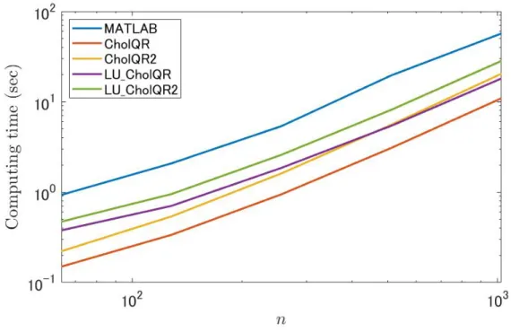
Figure 2.1: Comparison of the computation times for various n with m = 500,000 in Env. 1

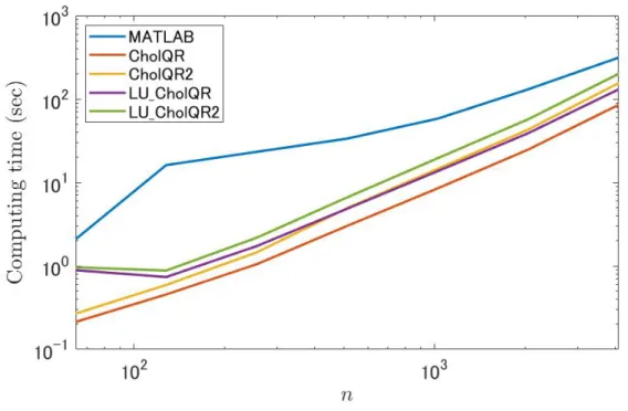
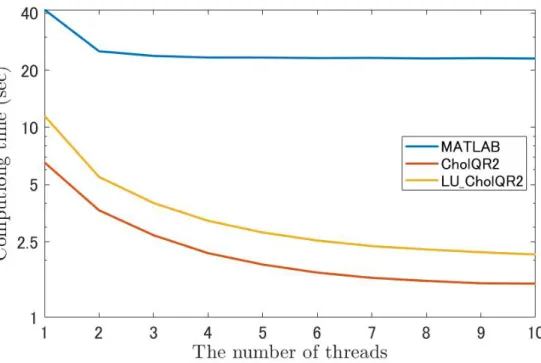
We first compare the computation time, and a test matrix A∈ Fm×n is generated using MAT-LAB’s function as A = rand(m,n). With respect to the computation times, Figs. 2.1 and 2.2 indicate that the proposed algorithms were faster than MATLAB’s qr function. Moreover, when n reached a certain size, the cost of preconditioning by LU decomposition was relatively less expensive, because the computational performance of LU decomposition was improved for larger n, especially in Env. 2. Next, we compared the strong-scalability of MATLAB’s qr function, CholeskyQR2, and LU-CholeskyQR2 algorithms in Env. 2. From Fig. 2.3, strong-scalability of LU-LU-CholeskyQR2 is superior to that of MATLAB’s QR, and comparable to that of CholeskyQR2.

Next we compare orthogonality and residual on Env. 1, and generate test matrices using Higham’s randsvd function [9] as

A = gallery(’randsvd’,[m,n],cnd,mode,m,n,1),

where cnd is a specified generalized condition number κ2(A), and mode can be selected as follows:

1. One large singular value. 2. One small singular value.

3. Geometrically distributed singular values. 4. Arithmetically distributed singular values.

(25)

Figure 2.2: Comparison of the computation times for various n with m = 1,000,000 in Env. 2

In numerical examples, we choose mode = 3 unless otherwise specified. As a standard Householder QR algorithm, we use MATLAB’s qr function for thin QR decomposition as

[Q,R] = qr(A,0).

For comparison on the orthogonality∥ ˆQTQˆ− I∥2 and the residual norms∥ ˆQ ˆR− A∥2 for computed

QR-factors, we use the Advanpix Multiprecision Computing Toolbox [15] for calculating them

precisely.

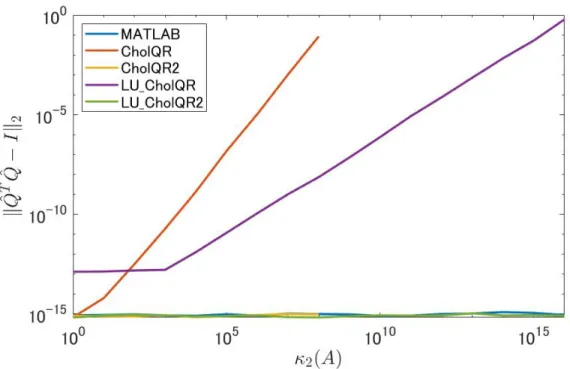
Figure 2.4 compares the orthogonality as ∥ ˆQTQˆ − I∥2, and Fig. 2.5 compares the residuals as

∥ ˆQ ˆR − A∥2. As can be seen, the proposed algorithms (LU-CholeskyQR and LU-CholeskyQR2)

run to completion even if κ2(A) >

√

u−1. Moreover, the Q-factors computed by LU-CholeskyQR are successfully refined by LU-CholeskyQR2 in terms of orthogonality. It should be noted that neither CholeskyQR nor CholeskyQR2 cannot produce QR-factors if κ2(A) >

√

u−1, as Cholesky decomposition of fl (ATA) breaks down. Both the orthogonality and the residual norms of the

computed QR-factors obtained by LU-CholeskyQR2 are comparable to the results produced by MATLAB’s qr function.

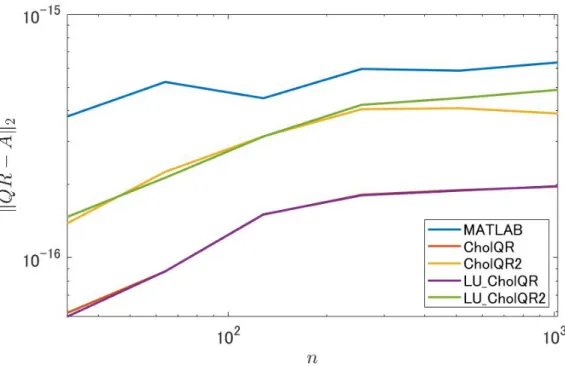
Moreover, Figs. 2.6 and 2.7 compare the orthogonality and the residual norms for m = 1024, 32 ≤ n ≤ 1024, and κ2(A) ≈ 107. Similar to the previous results, both the orthogonality and the

residual norms of the computed QR-factors obtained by LU-CholeskyQR2 are comparable to the results produced by MATLAB’s qr function.

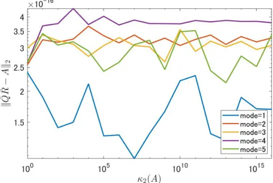
Furthermore, Figs. 2.8 and 2.9 display the orthogonality and the residual norms of the QR-factors computed by LU-CholeskyQR2, respectively, for all mode ∈ {1, 2, 3, 4, 5}. When κ2(A)≈ u−1, the

(26)

Figure 2.3: Comparison of the computation times for various threads with m = 1,000,000, n = 256 in Env. 2

2.3.2 Distributed memory computer environments

Finally, we show some numerical results on parallel distributed memory computers using RIKEN’s K computer and FUJITSU Supercomputer PRIMEHPC FX100. Computing times of the above algorithms are compared in the following two computational environments:

K computer CPU: SPARC6TM VIIIfx (8 cores), Memory: 16 GB / node

FX100 CPU: SPARC6TM XIfx (32 cores), Memory: 32 GB (HMC) / node

Here, we use mpifccpx as the Fujitsu C compiler command with MPI with the options -Kfast,parallel,openmp -SCALAPACK -SSL2BLAMP

on K computer and FX100 in common.

We generate m× n matrices whose elements are pseudo-random numbers uniformly distributed in the interval (0, 1) with m = 1,048,576, n = 256. Note that the generated test matrices are not ill-conditioned so that the Cholesky QR algorithms are applicable.

Tables 2.1 and 2.2 compare the computation times for the Householder QR algorithm (labeled ‘HouseholderQR’), CholeskyQR2, and LU-CholeskyQR2. We use the ScaLAPACK routines listed below:

Algorithm Major ScaLAPACK routines HouseholderQR pdgeqrf, pdorgqr

(27)

Figure 2.4: Comparison of the orthogonality∥ ˆQTQˆ− I∥2 for various κ2(A) with m = 1024, n = 128

in Env. 1

(28)

Figure 2.5: Comparison of the residual norms∥ ˆQ ˆR−A∥2for various κ2(A) with m = 1, 024, n = 128

in Env. 1

Figure 2.6: Comparison of the orthogonality ∥ ˆQTQˆ− I∥2 for various n with m = 1024, cnd = 107

(29)

Figure 2.7: Comparison of the residual norms ∥ ˆQ ˆR− A∥2 for various n with m = 1024, cnd = 107

in Env. 1

(30)

Figure 2.9: The residual norms∥ ˆQ ˆR− A∥2 for Algorithm I.5 (LU-CholeskyQR2) for various κ2(A)

with several singular value distributions with m = 1024, n = 128

Table 2.1: Comparison of computation times (sec) on RIKEN’s K computer (m = 1,048,576,

n = 256)

Algorithm\ # nodes 1 2 4 8 16 32 64 128 HouseholderQR 33.89 27.01 12.51 6.10 3.09 1.64 0.89 0.86 CholeskyQR2 7.78 2.58 1.29 0.67 0.36 0.20 0.14 0.12 LU-CholeskyQR2 23.93 12.39 6.24 2.79 1.48 0.82 0.50 0.43

Table 2.2: Comparison of computation times (sec) on FUJITSU FX100 (m = 1,048,576, n = 256) Algorithm \ # nodes 1 2 4 8 16 32 64

(31)

Chapter 3

Preconditioned Cholesky QR

algorithms in an oblique inner product

3.1 Introduction

In this chapter, we consider thin QR decomposition in an oblique inner product for full rank matrices

A ∈ Rm×n, m ≥ n and B ∈ Rm×m with B being positive definite. This decomposition produces

B-orthogonal columns Q∈ Rm×nand an upper triangular matrix R∈ Rn×nsuch that

A = QR, QTBQ = I, (3.1)

where I is the identity matrix. For the QR-factors computed by numerical computations, B-orthogonality as ∥QTBQ− I∥ and residual as ∥QR − A∥ are significant. Although CholeskyQR

has weak numerical stability, Cholesky QR is a fast algorithm employed for thin QR decomposi-tion [16]. In addidecomposi-tion, when CholeskyQR runs to compledecomposi-tion, we can refine B-orthogonality using CholeskyQR2 [16]. In Part I, we propose the fast and accurate numerical algorithms for this QR de-composition in an oblique inner product using Doolittle’s LU dede-composition. There are advantages in terms of B-orthogonality, residual, and computation times, that is shown in numerical examples.

3.2 Preliminaries

We first define the notation in Part I. Let F be a set of binary floating-point numbers, and let

u be the unit roundoﬀ (binary64: u = 2−53). The 2-norm of vector x = (xi) ∈ Rn and matrix

A = (aij)∈ Rm×n indicates that ∥x∥2 = v u u t∑n i=1 x2_i, ∥A∥2= max ∥x∥2=1 ∥Ax∥2.

Matrix A+denotes the Moore-Penrose pseudoinverse matrix of A; that is, A+= (ATA)−1AT. κ2(A)

is the condition number such that κ2(A) =∥A∥2∥A+∥2.

3.2.1 Cholesky QR algorithm

In this subsection, we first introduce Cholesky QR algorithms in an oblique inner product for

(32)

Algorithm I.6. CholeskyQR algorithm in an oblique inner product function [Q1, R1] = CholQR(A, B) C = A′∗ B ∗ A; % C ≈ ATBA R1 = chol(C); % C ≈ RT1R1 Q1= A/R1; % Q1 ≈ AR−11 end

Since this algorithm is implementable using Level-3 routines in basic linear algebra subprograms (BLAS) and linear algebra package (LAPACK), CholeskyQR achieves high performance on speed. However, the paper [16] reports numerical instability of CholeskyQR. For a matrix C as κ2(C)≳

u−1, Cholesky decomposition for C breaks down in many cases. Here, we have

κ2(ATBA)≤ κ2(A)2κ2(B). (3.2)

Therefore, even if matrices A and B are well-conditioned, there is possibility that C is ill-conditioned. This indicates that CholeskyQR has weak numerical stability.

3.2.2 Refinement of a Q-factor

Next, we consider the refinement after applying CholeskyQR for A and B. The following algorithm named CholeskyQR2 [16] refines B-orthogonality ∥QT_BQ_{− I∥}

2.

Algorithm I.7. CholeskyQR2 algorithm in an oblique inner product

function [Q2, R2] = CholQR2(A, B)

[Q1, R1] = CholQR(A, B);

[Q2, R] = CholQR(Q1, B);

R2 = R∗ R1;

end

For m≫ n, the cost of CholeskyQR2 is almost twice as much as that of CholeskyQR.

3.2.3 Shifted Cholesky QR algorithm

We introduce the shifted Cholesky QR algorithms [17] whose numerical stability is stronger than that of the standard Cholesky QR algorithms.

Algorithm I.8. Shifted CholeskyQR algorithm in an oblique inner product

function [Q1, R1] = sCholQR(A, B, s)

C = A′∗ B ∗ A;

R1= chol(C + s∗ I); % s is a positive constant

Q1 = A/R1;

(33)

Even if κ2(C) > u−1, κ2(C + sI)≤ u−1 is satisfied by the diagonal shift. In [17], the amount of

shift is calculated as

s≈ 11(2m√mn + n(n + 1))u∥A∥2₂∥B∥2. (3.3)

Similarly, the shifted CholeskyQR2 and shifted CholeskyQR3 are introduced as follows [17]:

Algorithm I.9. Shifted CholeskyQR2 algorithm in an oblique inner product

function [Q2, R2] = sCholQR2(A, B, s)

[Q1, R1] = sCholQR(A, B, s);

R2 = R∗ R1;

end

Algorithm I.10. Shifted CholeskyQR3 algorithm in an oblique inner product

function [Q3, R3] = sCholQR3(A, B)

[Q1, R1] = sCholQR(A, B, s);

[Q3, R] = CholQR2(Q1, B);

R3= R∗ R1;

end

3.3 LU-Cholesky QR algorithms in an oblique inner product

In this section, we propose the LU-Cholesky QR algorithm employed for thin QR decomposition in an oblique inner product. We focus on the preconditioning using numerical computations of Doolittle’s LU decomposition of a given matrix A such that

P A≈ ˆL ˆU ,

where ˆL is a unit lower triangular matrix, ˆU is an upper triangular matrix, and P is a permutation

matrix. It is known that ˆL tends to be fairly well-conditioned even if A is ill-conditioned.

We apply Doolittle’s LU decomposition to preconditioning of CholeskyQR.

Algorithm I.11. LU-CholeskyQR algorithm in an oblique inner product

(34)

If a given matrix A is ill-conditioned, κ2(A)≥ κ2(L), so that the point of this algorithm is that

κ2( ˆLTP BPTL)ˆ ≲ κ2(ATBA) is expected. Hence, even if a matrix A is ill-conditioned, the proposed

algorithm for A and B being κ2(B) < u−1 can run to completion.

Next, LU-CholesktQR2 algorithm is explained.

Algorithm I.12. LU-CholeskyQR2 algorithm in an oblique inner product

function [Q2, R2] = LU CholQR2(A, B)

[Q1, R1] = LU CholQR(A, B);

R2= R∗ R1;

end

LU-CholekyQR2 aims to refine B-orthogonality such as the original CholeskyQR2 algorithm introduced in Section 3.2.2.

3.4 Numerical results

Here, we provide the numerical results. Matrices A and B are generated by MATLAB as follows:

A = gallery(′randsvd′, [m, n], cndA, 3, m, n, 1), B = gallery(′randsvd′, m, cndB, 3, m, m, 1).

These matrices A and B satisfy κ2(A) ≈ cndA, κ2(B) ≈ cndB and ∥A∥2,∥B∥2 ≈ 1. Therefore, for

simplicity, we obtain the shift amount s in (3.3) as s ≈ 11(2m√mn + n(n + 1))u for sCholQR,

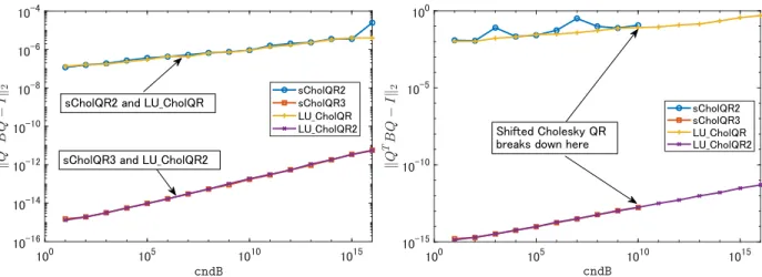
sCholQR2, and sCholQR3. Figure 7.2 compares B-orthogonality of the shifted Cholesky QR and LU-Cholesky QR algorithms for various κ2(B) for cndA = 109and cndA = 1014. The figure indicates

that the B-orthogonality of the Q-factor computed by the proposed algorithms is comparable to that computed by the shifted Cholesky QR. From right side in Fig. 7.2, although the standard Cholesky QR algorithms break down when κ2(B)≳ 1010 and cndA = 1014, LU-Choleksy QR algorithms can

be applied to ill-conditioned matrices.

Figure 3.2 compares residual of shifted Cholesky QR and LU-Cholesky QR algorithms for various

κ2(B) for cndA = 109 and cndA = 1014. The residual of the QR-factors computed by the proposed

algorithms is comparable to that computed by the shifted Cholesky QR.

Finally, we compare the computation times for the following random matrices generated by the MATLAB function; A = randn(m, n) and B = randn(m). The computation environment of the computer and MATLAB are as follows:

CPU: Intel Core i7-8550U, Memory: 16 GB, MATLAB R2019a

(35)

Figure 3.1: Comparison of B-orthogonality (m = 1024, n = 256, cndA = 109 (left) and cndA = 1014 (right)).

(36)

Figure 3.3: Comparison of computation times [sec] for various n. (m = 10, 000)

3.5 Conclusion for Part I

In Part I, we propose LU-Cholesky QR algorithms for thin QR decomposition to improve the robust-ness of existing Cholesky QR algorithms. Our investigations in Part I indicate that the proposed algorithms would eﬀectively work for ill-conditioned matrices while Cholesky QR algorithms, such as CholeskyQR and CholeskyQR2 would not be applicable.

With respect to computation time, the comparisons in our numerical examples reveal that

• LU-CholeskyQR2 is faster than the Householder QR algorithm on both the shared memory

computers and distributed memory computers used in Part I,

• the computation time for LU-CholeskyQR2 is approximately 1.5 times greater than that of

CholeskyQR2 on our shared memory computers, and

• the computation time for LU-CholeskyQR2 is between 3 and 5 times greater than that of

CholeskyQR2 on the distributed memory computers used in Part I.

With respect to the orthogonality and norms of residuals, LU-CholeskyQR2 is comparable to CholeskyQR2 and the Householder QR algorithm.

We also presented the results of rounding error analysis of the proposed algorithms in a similar way to the Cholesky QR algorithms.

(37)

Part II

(38)

Chapter 4

Introduction

4.1 Introduction

The goal of this chapter is to propose fast methods for proving the nonsingularity of a matrix

A∈ Rn×n using only numerical computations based on IEEE 754 [5]. To prove the nonsingularity of a given matrix, one of the following may be demonstrated:

• that the determinant is not zero, • that the matrix inverse exists, • that there are no zero eigenvalues.

If numerical computations are used for these approaches, rounding error problems arise. For ex-ample, we cannot obtain the exact determinant, inverse matrix, and eigenvalues due to the ac-cumulation of rounding errors. We aim to prove the nonsingularity of a given matrix using only floating-point arithmetic.

It is known that the matrix A is nonsingular if there exists a matrix R∈ Rn×n such that

∥RA − I∥ < 1, (4.1)

where I is the identity matrix. This theory is often used for computer-assisted proofs of nonsin-gularity of matrices. It is diﬃcult to rigorously compute ∥RA − I∥ using floating-point arithmetic due to rounding error problem. Therefore, an upper bound of∥RA − I∥ can be computed. Proving

∥RA − I∥ < 1 is also essential for verifying numerical computations for linear systems. Let a linear

system be Ax = b, x, b ∈ Rn _{and an approximate solution of Ax = b be ˆ}_{x. If}_{∥RA − I∥ < 1, then}

the upper bound of the error is bounded by

∥ˆx − x∥ ≤ ∥R(b − Aˆx)∥

1− ∥RA − I∥.

In Part II, we use the maximum norm and focus on how to obtain upper the bound of ∥RA − I∥_∞ using only floating-point arithmetic.

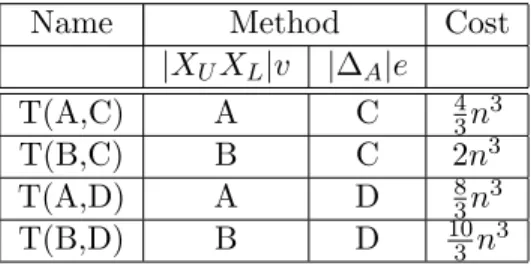
There are two strategies for setting R. One is using LU factors and their approximate inverses [18, 19, 20, 21]. Let ˆL and ˆU be the computed LU factors of P A, where P is a permutation

(39)

ˆ

U , respectively. Then, R is set by R := XUXLP . The second strategy is to compute R as the

approximate inverse of a matrix A directly [18, 19].

In this chapter, we propose four new methods for obtaining the upper bound of ∥RA − I∥_∞ by setting R := ( ˆL ˆU )−1P . These methods have advantages for proof of nonsingularity of interval

matrices. Numerical results illustrate their eﬃciency. In addition, the proposed methods often result in superior upper bounds of∥RA − I∥_∞although their computational cost is lower than that of previous studies.

The remainder of this chapter is organized as follows. We introduce the target problem and present an overview of previous studies in Section 4.2.1. In Section 4.2.2, we summarize notations and lemmas for rounding error analysis. In addition, we describe previous studies on obtaining the upper bound of ∥RA − I∥_∞. In Section 4.2.3, we introduce new methods and their extension to interval matrices with numerical examples. This study is related to [B1, C10–C22] in the list of publications.

4.2 Previous studies

4.2.1 Notation

Here, we introduce the notation used in Part II. Let F be a set of binary floating-point numbers as defined by IEEE Std. 754 [5]. Notations f l(·), fl_▽(·), and fl_△(·) indicate that all operations inside parentheses are evaluated using floating-point arithmetic with the following rounding modes: rounding to the nearest (roundTiesToEven), rounding downward (roundTowardNegative) and up-ward (roundToup-wardPositive), respectively. Let u be the unit roundoﬀ and us be the minimum

positive value in floating point numbers, for example, u = 2−53, us = 2−1074 for binary64 in IEEE

Std. 754. For x, y∈ Rn, the notation|x| is defined as |x| = (|x1|, |x2|, . . . , |xn|)T and x < y signifies

xi < yi for all i. This notation can easily be extended to matrices. E ∈ Fn×n and e ∈ Fn are an

n-by-n matrix and n-vector of ones, respectively, while matrices EL and EU are lower and upper

triangular matrices whose all elements are 1, respectively. As in Section 1.2.1, we also count the number of floating-point operations in flops1. For simplicity, we only use the maximum degree of a polynomial for flops. For example, the number of floating-point operations of a product of

A, B ∈ Fn×nis considered by 2n3flops excluding theO(n2) terms. For a matrix A∈ Rn×n, diag(A) represents the vector (a11, . . . , ann)T ∈ Rn. For A, B∈ Fn×n, a function max(A, B) returns a matrix

with the largest elements taken from A or B.

4.2.2 A priori error analysis

Here, we perform standard rounding error analysis for matrix multiplication, LU decomposition, and triangular systems. For A∈ Fn×n, suppose that matrices ˆL and ˆU are computed by several variants

of Gaussian elimination with partial pivoting, where pivoting information is stored in permutation matrix P such that ˆL ˆU ≈ P A.

Lemma II.1 ([13]). For A, B ∈ Fn×n, a computed result of matrix multiplication C := fl(AB) satisfies

|AB − C| ≤ nu|A||B| +nus

2 E.

(40)

Lemma II.1 applies to blocking strategies, however, it does not apply to more sophisticated methods, such as those proposed by Strassen [10], Coppersmith and Winograd [11], or Williams [12]. For example, given A ∈ Fm×n and B ∈ Fn×k, let C be the approximation of their product AB returned by using mk inner products in dimension n in any order of evaluation.

The following lemmas are related to the residual for LU decomposition and triangular systems. We introduce results from [14] with an underflow term from [18].

Lemma II.2 ([14] and [18]). For A∈ Fn×n, suppose that matrices ˆL and ˆU are the computed LU factor. If nu < 1, then, also in the presence of underflow,

ˆ

L ˆU− P A = ∆A, |∆A| ≤ nu|ˆL|| ˆU| +

us

1− nu(ne + diag(|U|))e

T_.

Lemma II.3 ([14] and [18]). Let matrix equation T X = B, where T ∈ Fn×n is a nonsingular triangular matrix, be solved by forward / backward substitution. If nu < 1, then the computed solution ˆX satisfies

T ˆX = B + ∆, |∆| ≤ nu|T || ˆX| + us

1− nu(nI + D)ET,

where D is the diagonal matrix of T . If T is a lower triangular matrix, then ET := EL. Otherwise,

ET := EU. If matrix T is a unit triangular matrix, then

|∆| ≤ nu|T || ˆX| + nus

1− nuET

is satisfied.

Lemma II.4 ([22, p. 145]). If T ={tij} is a nonsingular triangular matrix, then

|T−1| ≤ M(T )−1,

where the triangular matrix M (T ) ={mij} is the comparison matrix of T :

mij = { |tii|, i = j −|tij|, i ̸= j . 4.2.3 Verification methods

In this subsection, we introduce previous studies on computing the upper bound of∥RA−I∥_∞. First, we introduce verification methods for computing an approximate inverse matrix of A. Assuming that R is a computed inverse matrix, the computational cost of obtaining R is 2n3 flops. Then, an upper bound of|RA − I| can be obtained by

(41)

Algorithm II.1 (Oishi-Rump [18]). For A ∈ Fn×n, the following algorithm computes an upper bound of ∥RA − I∥_∞.

function res = Method1(A)

R = inv(A); % R is an approximate inverse of A

feature(′setround′,−inf); % Change the rounding mode to rounding downward S1 =|RA − I|;

feature(′setround′, inf); % Change the rounding mode to rounding upward S2 =|RA − I|;

S = max(S1, S2);

res = norm(S, inf); % res≥ ∥S∥_∞

end

Algorithm II.1 computes the approximate inverse performs matrix and performs two matrix multiplications. Therefore, the computational cost of Algorithm II.1 is 6n3 flops.

Here, we introduce a faster method. From Lemma II.1, an upper bound of |RA − I| can be obtained by

|RA − I|e ≤ fl(|RA − I|)e + (n + 1)u(|R|(|A|e) + e) +nus

2 Ee. Thus, we have an upper bound of ∥RA − I∥_∞ as

∥RA − I∥∞ = ∥|RA − I|e∥∞≤ ∥fl(|RA − I|)e + (n + 1)u(|R|(|A|e) + e)∥∞+ n2us/2

≤ ∥fl△(fl(|RA − I|)e + (n + 1)u(|R|(|A|e) + e)∥∞+ n2us/2). (4.3)

We introduce an algorithm based on (4.3) using directed rounding2_.

Algorithm II.2. Let A, R∈ Fn×n. This algorithm computes an upper bound of∥RA − I∥_∞

function res = Method2(A)

n = size(A, 1); e = ones(n, 1);

R = inv(A); % R is an approximate inverse of A S =|RA − I|;

feature(′setround′, inf); % Change the rounding mode to rounding upward T = Se + (n + 1)u(|R|(|A|e) + e) + n2us/2;

res = norm(T, inf);

end

Algorithm II.2 computes the approximate inverse matrix and performs matrix multiplication. The computational cost of Algorithm II.2 is 4n3 flops, which is smaller than that of Algorithm II.1. However, res obtained by Algorithm II.1 is often significantly smaller than that obtained by Algo-rithm II.2.

2

Thin QR分解に対する高精度数値計算法と行列方程式に対する精度保証付き数値計算の研究

芝 浦 工 業 大 学

博 士 学 位 論 文

Studies on Accurate Numerical Computations of

Thin QR Decomposition and Verified Numerical Computations

for Matrix Equations

Thin QR

分解に対する高精度数値計算法と行列方程式に対する

精度保証付き数値計算の研究

令和

2

年

3

月

Takeshi Terao

Abstract

Contents

Part I

Chapter 1

Introduction

1.1

Introduction

1.2

Background

Chapter 2

LU-Cholesky QR algorithms for thin

QR decomposition

2.1

Proposed algorithms

2.2

Rounding error analysis of the proposed algorithms

2.3

Numerical results

Chapter 3

Preconditioned Cholesky QR

algorithms in an oblique inner product

3.1

Introduction

3.2

Preliminaries

3.3

LU-Cholesky QR algorithms in an oblique inner product

3.4

Numerical results

3.5

Conclusion for Part I

Part II

Chapter 4

Introduction

4.1

Introduction

4.2

Previous studies

芝浦工業大学

博士学位論文