芝浦工業大学学術リポジトリ

(1)

New Methods of Tilt

Measurement for Applications in

Medical Devices

A DISSERTATION SUBMITTED TO THE

GRADUATE SCHOOL OF ENGINEERING AND SCIENCE OF SHIBAURA INSTITUTE OF TECHNOLOGY

by

DAO VIET HUNG

IN PARTIAL FULFILLMENT OF THE REQUIREMENTS FOR THE DEGREE OF

DOCTOR OF ENGINEERING

(2)

Acknowledgments

I owe a deep sense of gratitude to all kindnesses and supports for my studies. Like once said that no one succeeds all by themselves, the work would not have been completed without the help of many individuals.

First and foremost, I would like to send my deepest appreciation to my family for their spiritual support, which motivates and encourages me to accomplish the research successfully. Moreover, those achievements of mine could not be attained without the presence of my wife, who has always been by my side and has given me strength to overcome the diﬃculties during these three years of hard working.

I would like to express my gratitude to my supervisor, Professor Takashi Komeda, for his research orientation from the very beginning of my study, the guidelines, valuable advice, throughout the time of the research as well as his enthusiastic supervision and encouragement for the successful completion of this dissertation.

I would also like to thank Prof. Akihiko Hanafusa, Prof. Kazuhisa Ito, Prof. Akihiro Matsumoto, and Prof. Shinichiro Yamamoto in the review board for their perceptive comments on the thesis in view of the fact that these comments not only led to the enhancement of my work but also suggested new tendencies for the research development. I truly appreciate the reviewers for dedicating their time to help me to successfully complete the study.

(3)

members of Shibaura Institute of Technology, particularly personnel of the Student Aﬀairs Section and Graduate School Section for their kind help and endless support. In addition, I am very grateful to my Japanese friends who have willingly helped me to become familiar with a new place, way of life and language here in Japan. Thanks to their moral support, I had more time to work at a high level without being distracted.

Furthermore, immeasurable appreciation is extended to the Olympus company for providing me a chance to get the use of endoscopic de-vices, together with Mr. Keita Suzuki who gave me beneﬁcial advice related to endoscopic surgery. Following that, I would like to acknowl-edge the support of my friend, Mr. Lawrence E. Walker, who helped me proof checking to detect any language errors. My publications would not have been accomplished without his assistance.

Last but not least, I am very grateful to my kind friends and colleagues who are one way or another shared their support and understanding spirit, thank you all.

Saitama, September 2, 2016

(4)

Abstract

Tilt measurement is useful for a variety of applications. In medical ﬁeld, the tilt angles can be used to determine inclinations of the hu-man bodies, angles of huhu-man joints, as well as orientations of surgical devices. Tilt measurement is also necessary for consumer electronics, industrial electronics, avionics, and other applications in both civil and military, which require the inclinations of an object with respect to either vertical axis or horizontal plane.

Measuring the tilt angles with inertial sensors is a well-known tech-nique. An accelerometer can sense any change in a linear velocity as well as measuring the constant gravitational acceleration. Hence, by using a triaxial acceleration sensor, three orthogonal projections of the gravity vector onto the sensor frame can be determined for computing the tilt angles. The calculation formulas depend on the deﬁnition of the tilt angles which can be classiﬁed into some major types.

Both analog and digital accelerometers are commonly utilized for mea-suring the tilt angles. Digital accelerometers are a good choice in many cases, whereas an analog accelerometer could be necessary when the system requirements are beyond the capability of the digital sensor. However, when using the analog sensors, the eﬀects of the electromag-netic interference must be taken into account.

(5)

The objectives of this work are to partially solve the limitations of the tilt measurement technique in the medical field. The whole work is divided into four elemental studies. The first three studies are pro-posed based on the same idea that is the interference cancellation can be achieved by changing the mounting orientation of the acceleration sensors. In each study, a rotation matrix is proposed to rotate the sen-sor frame and convert the calculation formulas. This change allows computing the tilt angles from the differences between the voltages of three sensor outputs. Thus, an advantage of the differential signaling technique, that is interference immunity, is taken within the single-ended systems. In spite of using the same mechanism, each study plays a dedicated role because they improve three major types of the tilt components.

In the last study, a new sensor-fusion method is proposed to reduce the eﬀects of motion on the tilt angles. The key algorithm is a so-called predict-and-choose process which combines the accelerometer readings and the output data of a triaxial gyroscope. During the dynamic states, this process predicts three gravitational components to estimate the tilt angles. Therefore, the dependence of the computed results on the motion can be reduced.

(6)

List of Figures

2.1 A rotation about Z-axis: (a) active rotation and (b) passive rotation 8 2.2 Two types of rotation: (a) extrinsic rotation and (b) intrinsic rotation 10 2.3 Deﬁnition of the tilt angles based on the yaw-pitch-roll order Euler

angles: (a) initial position and (b) two tilt angles . . . 12 2.4 Deﬁnition of the tilt in which two components are interchangeable 13 2.5 Another deﬁnition of the tilt based on the non-Euler angles: (a)

the tilt has two components and (b) only one inclination is used . 13 2.6 Coordinate system of the measured object and the conventional

mounting method for accelerometers . . . 14 2.7 Calculation of the tilt when using the Euler angles . . . 16 2.8 Calculation of the tilt when using the non-Euler angles . . . 17 2.9 Inﬂuence of digital switching noise and crosstalk in digital

ac-celerometers . . . 18 2.10 External noise and the eﬀects on the computed tilt angles . . . 20 2.11 Diﬀerences between the gravitational components and the

accelerom-eter readings when the linear acceleration is nonzero . . . 21 2.12 Quantifying the linear acceleration by comparing magnitude of F

and g: (a) there is no confusion and (b) appearance of the error . 22 3.1 The deﬁnition of the proposed orientation in measuring the pitch

angle . . . 25 3.2 Main components of the simulation model . . . 29 3.3 Precise results of both methods when there is no noise . . . 30 3.4 Angle errors under the eﬀects of the external noise: nRM S = 50 mV 30

(11)

LIST OF FIGURES

3.6 Errors in the computed pitch angles in diﬀerent ranges of the orig-inal pitch angle . . . 33 3.7 Errors in the computed roll angles in diﬀerent ranges of the original

pitch angle . . . 33 3.8 Adapter for altering the attachment of the accelerometer . . . 35 3.9 Analog accelerometer and the three-core twisted cable . . . 36 3.10 Noises in the connection wires and the diﬀerence between them . 37 3.11 Stability of the pitch angle computed by proposed method and the

fluctuations of the remaining angles . . . 37 3.12 Differences between the errors in the computed pitch angles . . . 39 3.13 Differences between the errors in the computed roll angles . . . . 39 4.1 Three major units in the hardware system . . . 43 4.2 The definition of the proposed orientation in measuring the roll angle 44 4.3 One common-mode noise source and six differential-mode noise

sources in the simulation model . . . 48 4.4 Both methods compute the angles precisely when there is no noise 49 4.5 Angle errors under the eﬀects of the external noise: nc = 50 mV

and nd= 0.5 mV . . . . 49

4.6 Angle errors under the eﬀects of the external noise: nc= 100 mV

and nd= 1 mV . . . 50

4.7 Errors in the computed roll angles in diﬀerent ranges of the original pitch angle . . . 52 4.8 Errors in the computed pitch angles in diﬀerent ranges of the

orig-inal pitch angle . . . 52 4.9 Mechanical system in experiments: (a) sensor mounting frame and

(b) rotation frame . . . 53 4.10 Measured noises in single-ended signals and diﬀerential signals . . 54 4.11 Diﬀerences between the angles of two methods when ΦO = −45

deg and ΘO = 80 deg . . . 55

(12)

LIST OF FIGURES

5.1 The deﬁnition of the proposed orientation in measuring both

non-Euler tilt angles . . . 61

6.1 System overview with key components and key processes in the basic application . . . 72

6.2 The tip of the ﬂexible endoscope: (a) position of the IMU and (b) three elemental rotations . . . 73

6.3 Sensor-fusion in the predict-and-choose process . . . 74

6.4 Gravitational vector changes caused by each rotation component: (a) rotation about Z-axis changes gx and gy; (b) rotation about the X-axis changes gy and gz; and the rotation about the Y-axis changes gz and gx . . . 75

6.5 Generating the simulation data in the virtual IMU: (a) schematic diagram of virtual IMU and (b) original tilt angles for conditions (iii) and (iv), Φ changes as a sine function and Θ changes as a linear function . . . 80

6.6 Simulation results under condition (ii), linear acceleration only: akmax = 3 m/s 2 _{and ω = 0 . . . .} ₈₁

6.7 Simulation results under condition (iii), rotation with small back-ground vibration: akmax = 0.5 m/s 2 _{and ω}̸= 0 . . . 82

6.8 Simulation results under condition (iv), combined linear accelera-tion and rotaaccelera-tion: akmax = 3 m/s 2 _{and ω} _{̸= 0 . . . 82}

6.9 Simulation results under condition (iv), combined linear accelera-tion and rotaaccelera-tion: akmax = 10 m/s 2 _{and ω} _{̸= 0 . . . 83}

6.10 Rotation frame in the experiments . . . 83

6.11 Experimental results when the motion noise is small . . . 85

6.12 Experimental results under the strong motion . . . 85

6.13 Using the output angles of both methods for horizon stabilization under some conditions: (a) static state, (b) weak motion, (c) strong motion, and (d) continuous strong motion . . . 86

(13)

List of Tables

3.1 Dependence of angle errors (mean and SD) on the range of the pitch angle . . . 32 3.2 Speciﬁcations of the chosen accelerometer, KXR94-2050 . . . 34 3.3 Errors (mean and SD) in computed angles on some speciﬁc

orien-tations . . . 38 4.1 Mean values and SD of angle errors on some speciﬁc ranges of the

(14)

Nomenclature

Roman Symbols

a linear acceleration vector

aX orthogonal projection of a onto the X-axis

aY orthogonal projection of a onto the Y-axis

aZ orthogonal projection of a onto the Z-axis

F sum of g and a

FX orthogonal projection of F onto the X-axis

FY orthogonal projection of F onto the Y-axis

FZ orthogonal projection of F onto the Z-axis

g standard gravity, about 9.8m/s2 g gravitational vector

gX orthogonal projection of g onto the X-axis

gx orthogonal projection of g onto the x-axis

gY orthogonal projection of g onto the Y-axis

gy orthogonal projection of g onto the y-axis

(15)

NOMENCLATURE

gz orthogonal projection of g onto the z-axis

n external noise

nx noise in the measured signal of the x-axis

ny noise in the measured signal of the y-axis

nz noise in the measured signal of the z-axis

O1O2O3 coordinate system of the measured object

rF downsampling ratio for accelerometer

rω downsampling ratio for gyroscope

R rotation matrix

RX(α) elemental rotation about the X-axis by α

RY(β) elemental rotation about the Y-axis by β

RZ(γ) elemental rotation about the Z-axis by γ

s accelerometer sensitivity

Ux output voltage of the sensor on the x-axis

Uy output voltage of the sensor on the y-axis

Uz output voltage of the sensor on the z-axis

v, v’ column vectors which represent coordinates of a point XY Z conventional mounting orientation of the accelerometers

xyz proposed mounting orientation of the accelerometers Greek Symbols

α, β, γ rotation angles

(16)

NOMENCLATURE

ωX angular velocity about the X-axis

ωY angular velocity about the Y-axis

ωZ angular velocity about the Z-axis

Φ the third elemental rotations of ZYX convention Euler angles Ψ the ﬁrst elemental rotations of ZYX convention Euler angles Θ the second elemental rotations of ZYX convention Euler angles θ1, θ2 two tilt angles when non-Euler angles are used

Superscripts a active Subscripts C conventional method c common-mode d diﬀerential-mode k x, y, z, or all of them

n time point with labels in chronological order O original (angles)

P proposed method Acronyms

ADC analog-to-digital converter CMRR common-mode rejection ratio DAQ data acquisition

(17)

NOMENCLATURE

EMI electromagnetic interference f video frame

FS full scale

IC integrated circuit

IMU inertial measurement unit

MEMS micro-electro-mechanical systems

NOSCAR Natural Oriﬁce Surgery Consortium for Assessment and Research NOTES natural oriﬁce translumenal endoscopic surgery

RFI radio frequency interference RMS root mean square

(18)

Chapter 1 Introduction

This chapter provides an outline of the whole work. In the ﬁrst section, an overview of the tilt measurement technique and its challenges are introduced. This is the basis for the research objectives in the following section. After that, the outstanding results of each elemental study are summarized to highlight the contributions of the work. Finally, a listing of all chapters provides a panoramic view of the entire study.

1.1 Overview

In recent years, the development of micro-electro-mechanical systems (MEMS) technology allows utilizing the inertial sensors in more and more applications, including tilt measurement. A low cost three-axis MEMS accelerometer, with a size of a few millimeters, can measure three Cartesian components of any ac-celeration. In the static or quasi-static conditions, these components are three elements of the gravitational vector, by which the tilt angles can be computed with trigonometric formulas. Because of the small size and ease of use, the MEMS accelerometers are not only integrated into new designs, but also used to upgrade the existing systems.

(19)

1.2 Objectives

many studies have focused on sensor calibration, sensor-fusion, and calculation algorithm to reduce the influence of these intrinsic limitations. An analog ac-celerometer can overcome some common limitations of the digital sensors. How-ever, when using the analog accelerometer, we face another challenge: interference susceptibility. Electromagnetic interference (EMI) can cause unwanted signals in transmission lines, and therefore disturb the final results. Although prevailing methods of interference reduction can effectively suppress the external noise, al-most all solutions require additional hardware or software or both of them, which could limit the applicability of the measurement system. The last challenge is the highest barrier in tilt measurement: effects of motion. According to the above mechanism, when vibration or movement appears, the accelerometer readings are no longer the gravitational components. In this case, additional processes or sen-sors are necessary to maintain the measurement accuracy. However, all of them have their own advantages and drawbacks. In general, there is always the need for developing the new methods which address the above limitations in the new way to expand the applicability of the tilt measurement systems.

1.2 Objectives

The objectives of this work are to partially solve the limitations of the tilt mea-surement technique in the medical field. The whole work consists of four elemental studies. The first three studies address the limitation of interference susceptibility of the analog accelerometers for expanding the applicability. Meanwhile, reducing the effects of motion on the tilt angles is taken into account in the last study.

(20)

1.3 Contributions

In the fourth study, the eﬀects of motion on the tilt angles are reduced by a new sensor-fusion method. This method allows estimating three gravitational components under all conditions. The key algorithm is a so-called predict-and-choose process which combines the output data of an accelerometer and a gyro-scope. The calculation algorithm guarantees that even in highly dynamic testing conditions, the estimated angles are reliable without any cumulative error. This study is developed to be applied in new surgical devices, particularly for natural oriﬁce translumenal endoscopic surgery (NOTES) systems.

Because of time and equipment constraints, the scope of the whole work is limited to be applied in the initially expected area, the medical field. The applica-tions would be expanded if further studies are conducted under other condiapplica-tions with dedicated measurement systems. Although this prediction has not been val-idated, the author believes that the idea of the first three studies can be utilized to enhance the EMI immunity and reduce the hardware complexity for many applications in a variety of fields.

1.3 Contributions

This work contributes three methods of EMI reduction and a method of sensor-fusion to enhance the accuracy of the tilt measurement systems. In order to highlight the difference among the first three methods, the definition of the tilt should be briefly clarified.

(21)

1.3 Contributions

The main contributions of this work are listed below:

EMI reduction in measuring the pitch angle By proposing a so-called pitch-improved rotation matrix (RΘ) to deﬁne a new mounting orientation for

the accelerometers, the author achieved a new measurement method in which the pitch angle can be measured without any error caused by EMI. The experimen-tal results showed that the error in the pitch angle was reduced 2–20 times, in comparison with the conventional method. Hence, the second angle of the ZYX convention Euler angles was improved.

EMI reduction in measuring the roll angle In this study, the author also proposed a so-called roll-improved rotation matrix (RΦ) to deﬁne a new mounting

orientation for the accelerometers. Then, the new method was validated by an upgraded simulation model and a new experimental system. The results showed that by this method, the error in the roll angle was reduced 5–22.5 times. Con-sequently, the third angle of the ZYX convention Euler angles was signiﬁcantly improved.

EMI reduction in measuring both non-Euler angles In the third study, the author theoretically proposed a solution to improve the two interchangeable tilt components simultaneously by a rotation matrix, Rθ1,2. After this change,

both non-Euler tilt angles can be immune to EMI at the same time, instead of only one angle as in the two above studies. Additionally, some alternative solutions for rotating the sensor were also proposed. Each of them rotates the sensor frame in a diﬀerent way. Thus, the mechanical attachment in each application will be more ﬂexible.

(22)

1.4 Structure of This Work

has smaller errors, smoother angle changes, and a smaller delay time, although the complexity of the hardware is almost unchanged.

The methods in the first three contributions have a common outstanding advantage that is the external EMI can be rejected without the need for any additional component or extra process. The EMI cancellation mechanism of the balanced lines has been achieved, although the proposed systems are single-ended. In other words, the author’s designs take an advantage of the differential signaling technique without the need for differential accelerometers, additional connection wires, and other necessary components of the differential systems. In conclusion, a totally new idea of EMI reduction in tilt measurement has been proposed, developed, and validated. This idea may be a good solution for many applications; particularly when the sensor is far from the processing circuit, the whole system works in a strong noise environment, and the size of all components should be kept to a minimum.

1.4 Structure of This Work

This dissertation is composed of seven chapters. Chapter 1 has provided the outline of the whole work. The next chapters are listed below:

Chapter 2 summarizes a technical background of the tilt measurement tech-nique and reviews the related studies. The content of this chapter includes: rotation and mathematical representation, tilt deﬁnition and angle calculation, and the common limitations of tilt measurement with inertial sensors. Simulta-neously, many related studies are reviewed.

Chapter 3 describes the new method of interference reduction in measuring the pitch angle with analog accelerometers. The structure of this chapter is similar to a scientiﬁc research articles, including descriptions of the method, simulation steps, and experiments processes.

(23)

1.4 Structure of This Work

structure of this chapter is similar to chapter 2. However, the objectives and implements of the two studies are diﬀerent.

Chapter 5 brieﬂy introduces the method that simultaneously improves the noise immunity of both non-Euler angles. Only equations are formulated here because there is no change in the validation method. This chapter also provides overall evaluations of the three presented studies and develops some alternative mounting solutions.

Chapter 6 presents the new method for estimating the tilt angles of endo-scopic images. Here, the new sensor-fusion method that combines the data of an accelerometer and a gyroscope is proposed. The results are evaluated by being applied in a well-known application, endoscopic horizon stabilization.

(24)

Chapter 2 Technical Background and

Literature Review

This chapter presents an overview of tilt measurement and reviews the related studies. In the first section, the fundamental of rotation and mathematical repre-sentations are briefly presented. This part provides the most important concepts and equations for the whole work. In the next section, a variety of the tilt definitions in many studies are reviewed. Conventional methods of tilt sensing with inertial sensors are also described in this part. The last section summa-rizes major challenges in tilt measurement, including limitations of the sensor and limitations of the calculation algorithm. Some prevailing solutions are also introduced to clarify the novelty of the contributions in this work.

2.1 Rotation and Representation

2.1.1 Basic Concepts

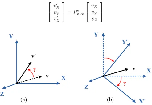
In three dimensions, any rotation of a point about a reference frame can be performed by a 3× 3 rotation matrix. The rotation, therefore, can be expressed by an equation, as in Eqn. (2.1). Here, the rotation matrix Ra _{rotates the point}

(25)

2.1 Rotation and Representation

frame is XYZ. In some cases, row vectors can also be used if the positions of Ra and v in the matrix multiplication are interchanged. The superscript a in Ra denotes the active rotation (alibi transformation) in which the point is moved while the reference frame is ﬁxed [32], as depicted in Fig. 2.1(a). In many cases, the passive rotation (alias transformation) is preferred. Here, the point (or vector v) is ﬁxed while the reference frame (XYZ) moves in the opposite direction, as in Fig. 2.1(b). This representation is very popular in engineering, when sensors are placed on the moving parts.

  v ′ X v_Y′ v_Z′   = Ra 3×3   vvXY vZ   (2.1) X Y v v' X Y v X' Y' γ γ (b) (a) Z Z

Figure 2.1: A rotation about Z-axis: (a) active rotation and (b) passive rotation Every rotation can be achieved by composing three elemental rotations which are the rotations about three axes of the Cartesian coordinate system. Equiv-alently, the rotation matrix Ra _{can be decomposed as the product of three}

(26)

2.1 Rotation and Representation

observing in the negative direction of the corresponding rotation axes.

Ra_X(α) =   10 cos α0 − sin α0 0 sin α cos α   (2.2) Ra_Y(β) =   cos β0 0 sin β1 0 − sin β 0 cos β   (2.3) Ra_Z(γ) = 

 cos γsin γ − sin γ 0cos γ 0

0 0 1



 (2.4)

When composing the above matrices, the position of the factors in the mul-tiplication determines the order in the rotation sequence. Before distinguishing this order, there are two terms should be clarified: extrinsic rotation and intrinsic rotation. Extrinsic rotations are rotations about the axes of the fixed coordinate system as depicted in Fig. 2.2(a), whereas intrinsic rotations are rotations about the axes of the rotating coordinate system, as in Fig. 2.2(b). The rotating coordi-nate system is initially aligned with the fixed one; however, its orientation changes after each elemental rotation [24]. Equation (2.5) is an example in which: if the rotations are intrinsic, the rotation order is X-Y-Z; meanwhile, if the rotations are extrinsic, the order is inverted. In the active rotations, because the reference frame is fixed, the extrinsic rotation is commonly used for representation. In Eqn. (2.5), elements of Ra _{are calculated from the trigonometric functions of the}

rotation angles. Here, s is the abbreviation of the sine function (e.g., sα is sin α),

while c is the abbreviation of the cosine function.

(27)

2.1 Rotation and Representation X Y X Y Z≡Z1 X1 Z2 X1 X2 Y1 Y2 Y1 Z≡Z1 RZ RY (a) (b) X Y X Y Z≡Z1 Y1 X1 Y1≡Y2 Z2 X1 X2 RZ RY Z≡Z1

Figure 2.2: Two types of rotation: (a) extrinsic rotation and (b) intrinsic rotation

2.1.2 Rotation of Sensors

(28)

2.2 Overview of Tilt Measurement

rotation matrices, as expressed in Eqn. (2.6), Eqn. (2.7), and Eqn. (2.8).

RX(α) =   10 cos α0 sin α0 0 − sin α cos α   (2.6) RY(β) =   cos β0 01 − sin β0 sin β 0 cos β   (2.7) RZ(γ) = 

 _{− sin γ cos γ 0}cos γ sin γ 0

0 0 1



 (2.8)

The composition in Eqn. (2.9) represents a Z-Y-X passive rotation sequence. The previously mentioned extrinsic rotations (active) become intrinsic rotations (passive) in this equation because the sensors are rotated about the axes of them-selves. This rotation sequence is widely known as the yaw-pitch-roll order or ZYX convention Euler angles which is commonly used in orientation measurement; more details are described in the next sections.

R = RX(α)RY(β)RZ(γ) =   sαsβccγβc− cγ αsγ sαsβscγβs+ cγ αcγ s−sαcββ cαsβcγ+ sαsγ cαsβsγ− sαcγ cαcβ   (2.9)

2.2 Overview of Tilt Measurement

2.2.1 Definitions of the Tilt Angles

There are two common methods to deﬁne the tilt of an object. In the ﬁrst method, two of the three Euler angles in yaw-pitch-roll sequence, namely roll and pitch, are used to represent the tilt of an object with respect to the horizontal plane [15, 20, 37], as depicted in Fig. 2.3. The initial position of the sensor, with the positive O3-axis in the vertical downward direction, is considered as the reference

(29)

2.2 Overview of Tilt Measurement 3rd Roll, Φ 1st Yaw, Ψ 2nd Pitch, Θ O2 O1 O3 O'2 O'1 O'3 O2 O1 O3 Φ Θ (b) (a)

Figure 2.3: Deﬁnition of the tilt angles based on the yaw-pitch-roll order Euler angles: (a) initial position and (b) two tilt angles

zero in Fig. 2.3), pitch (Θ) changes the inclination of the O1-axis, and roll (Φ)

is the rotation angle of the object about the moving O1-axis [13]. Since the two

angle play diﬀerent roles, they are not interchangeable.

In the second method, two components of the tilt are deﬁned as shown in Fig. 2.4. Here, one angle (θ1) is the inclination of the O1-axis, while another

one (θ2) is the inclination of the O2-axis, with respect to the horizontal plane

[27, 28, 45]. This deﬁnition is not based on any rotation sequence; therefore, the roles of the two components are interchangeable. When being compared with the Euler angles, θ1 seem to be same as Θ. In contrast, θ2 is really diﬀerent from Φ,

particularly when |Θ| increases to 90 deg.

In some studies, a similar deﬁnition of θ1,2 can be found. In Fig. 2.5(a), the

tilt components (θ′₁ and θ′₂) are deﬁned as the angles of the O1- and O2-axes with

(30)

2.2 Overview of Tilt Measurement O'2 O'₁ O'3 l1 l2 θ1 θ₂

Figure 2.4: Deﬁnition of the tilt in which two components are interchangeable

O'2 O'1 O'3 θ'1 θ'2 O'2 O'1 O'3 θ3 (b) (a)

(31)

θ′_1,2, and θ3 are called non-Euler angles. Although there are some diﬀerences

between their deﬁnitions and applications; the values of θ1,2, θ1,2′ , and θ3 can be

calculated by the same method. Therefore, in this work, only calculations of θ1

and θ2 are taken into account.

2.2.2 Conventional Method of Tilt Measurement

2.2.2.1 Sensors and the Mounting Orientation

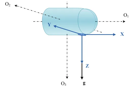
Tilt measurement with triaxial accelerometers is a well-known technique. The basic concept is that the tilt angles can be calculated from three components of the gravitational vector (g). In general, the mounting position of the sensor is customizable as long as their coordinate axes are parallel to those of the measured object, as shown in Fig. 2.6. Hence, the tilt of the sensor is also the inclination of the measured object. During static or quasi-static conditions, the tilt angles are calculated from absolute voltages of the sensor outputs; the formulas depend on which type of angles is used to deﬁne the tilt.

X

Z

Y

O

2

O

₁

O

3

g

(32)

2.2.2.2 Using the Euler Angles

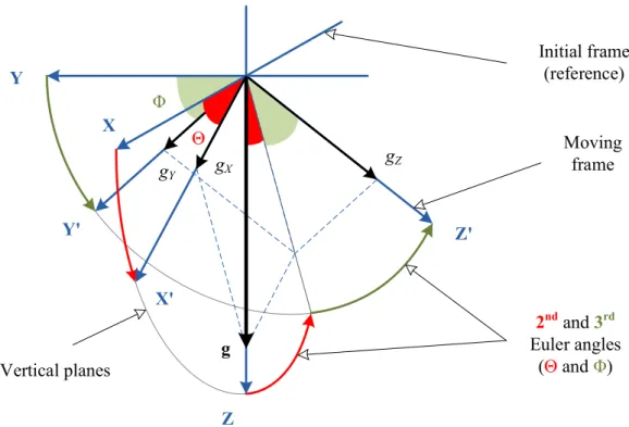
When using the Euler angles, calculation of the tilt is built from the rotation sequence. As mentioned in Sec. 2.1.2, the rotation matrix of the yaw-pitch-roll order (ZYX convention) Euler angles is expressed in Eqn. (2.9). Because the Z-axis of the reference frame points vertically downward, the gravitational vector is initially represented by a column vector that is [0 0 1]T_{. Thus, when the rotation}

sequence changes the orientation of the sensor, new coordinates of g are calculated by Eqn. (2.10) and then by Eqn. (2.11). Here, g has been normalized to make sure the rigor of the equation.

g = RZY X   00 1   (2.10) 1 |g|   ggXY gZ   = 

 cos Θ sin Φ− sin Θ cos Θ cos Φ



 (2.11)

On the basis of Eqn. (2.11), the value of Φ can be computed by Eqn. (2.12) and Θ is computed in Eqn. (2.13). These calculations can also be built from Fig. 2.7. In Eqn. (2.12), the arctan 2 function (with two arguments) is used instead of the arctan function (only one argument) to return the appropriate quadrant of the computed angle. The arctan 2 function can gather information on the signs of the two inputs and the output of the tradition arctan function, whose range is (−π/2, +π/2), to return the correct result in the range of (−π, +π).

(33)

2.2 Overview of Tilt Measurement g Y X Z X' Y' _Z' Initial frame (reference) Moving frame 2ndand 3rd Euler angles (Θ andΦ) gX gY gZ Θ Φ Vertical planes

Figure 2.7: Calculation of the tilt when using the Euler angles

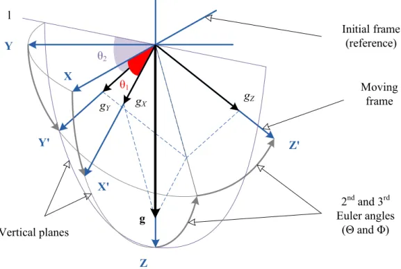
2.2.2.3 Using the Non-Euler Angles

Because the non-Euler angles are deﬁned by the geometric relations, the calcula-tion of the tilt is built visually. In Fig. 2.8, the sum of θ1 and the angle between

gX and g is 90 deg. Hence, θ1 can be computed by Eqn. (2.14). Here, in order

to make the form of Eqn. (2.14) be same as Eqn. (2.13), a minus sign is added. In other works, this sign could be changed, depending on the convention of the author. Similarly, θ2 can be determined by Eqn. (2.15). When the tilt angles are

deﬁned by the remaining methods (see Fig. 2.5), their values can be calculated by the same type of equation or computed from θ1 and θ2.

(34)

2.3 Major Challenges and Prevailing Solutions g Y X Z θ1 θ2 X' Y' _Z' Initial frame (reference) Moving frame gX gY gZ 2ndand 3rd Euler angles (Θ and Φ) l Vertical planes

Figure 2.8: Calculation of the tilt when using the non-Euler angles

2.3 Major Challenges and Prevailing Solutions

2.3.1 Limitations of Digital Accelerometers

Both analog and digital accelerometers are commonly utilized for measuring the tilt angles. Because of the convenience and the EMI immunity, the digital ac-celerometers are good choices in many applications. However, this type of the acceleration sensor has certain limitations.

(35)

2.3 Major Challenges and Prevailing Solutions

data need to be synchronized with an external clock source [20], the precise timing may not be guaranteed. Another problem is the digital switching noise in analog units (inside the MEMS) caused by sharing power and ground with digital units on a common substrate [35]. Figure 2.9 demonstrates the eﬀects in a digital accelerometer which is similar to a mixed-mode IC. Because the connection wires have resistances (2× Rwire), any fast transient in the digital signals will cause a

ripple in both common power source and ground point of the MEMS. In addition, there is a coupling eﬀect between the digital and analog units. Thus, the sensitive portions in the analog units may be disturbed, and therefore the error could be generated. Data Clock R_wire R_wire 3.3 V 0 V 3.3 V 0 V 3.3 V 0 V MEMS Analog units Digital units Processing circuit 3.3 V 0 V

Figure 2.9: Inﬂuence of digital switching noise and crosstalk in digital accelerom-eters

2.3.2 Advantages and Drawbacks of Analog Sensors

(36)

the intrinsic noise of the accelerometers itself could reduce the eﬀective resolution of the output data, this should be less a problem when more advanced sensors are used. This type of the accelerometer also has another advantage that is to allow processing the output signals in analog form [6]. In this case, the response speed can be maximized and the tilt can be determined without any quantization error. However, single-ended signals are very sensitive to electromagnetic interference presents on connection wires [42]. Therefore, EMI suppression is important if we want to take the full advantage of the analog accelerometers.

EMI can be reduced by many methods. Some common solutions are intro-duced in [46]. One of the simplest methods of EMI reduction is using filters. However, the filters always cause time delay, and therefore limit the bandwidth of the output signals. Figure 2.10 demonstrates an example in which the exter-nal noise in sensor sigexter-nals (three upper graphs) causes significant errors in the unfiltered output angle (fourth graph). Meanwhile, when a digital filter is used, the disturbance is almost rejected (last graph). However, the required sample for filtering is up to 200 when using a moving average filter. This could cause a remarkable time delay and should be avoided in many cases. Other methods are using shielded cables, shielding system, and preprocessors. They can isolate the analog circuits from the external EMI or convert the signals to other forms be-fore transmitting. However, these methods are not suitable when the installment space must be minimized, as in [20].

2.3.3 Limitations of the Measurement Method

Tilt measurement with accelerometers is based on a vital assumption that is the sensors are static or quasi-static. When there is no movement, the accelerometer can exactly measure three components (gX, gY, and gZ) of the gravitational

(37)

2.3 Major Challenges and Prevailing Solutions 0 10 20 -0.5 0 0.5 N o is e o n X (V ) 0 10 20 -0.5 0 0.5 N o is e o n Y (V ) 0 10 20 -0.5 0 0.5 N o is e o n Z (V ) 0 10 20 -35 15 65 U n filte re d Φ (d eg ) 0 10 20 -35 15 65 Time (ms) F ilte re d Φ (d eg )

Figure 2.10: External noise and the eﬀects on the computed tilt angles

angles could not be precise under the dynamic conditions. Hence, there is a need for special algorithms, additional sensors, or both of them.

(38)

g

X

Y

Z

g

X

g

Y

g

Z

F

X

F

Y

F

Z

a

F

Figure 2.11: Diﬀerences between the gravitational components and the accelerom-eter readings when the linear acceleration is nonzero

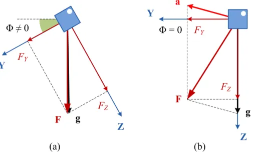
distinguish two values of Φ. The problem is clearly depicted in Figure 2.12(b) in which F is diﬀerent from g while |F| completely equals |g|. In this case, although the sensor is aligned horizontally, its readings are same as the sensor data in Figure 2.12(a), when Φ =−30 deg. Another study of endoscopic horizon stabilization was conducted by Warren et al. [47] in which the algorithm is based on that of H¨oller et al. Hence, both studies could have a same limitation.

(39)

2.4 Conclusion

Φ = 0

F

a

F

Y

F

Z

(b)

g

Z

Φ ≠ 0

F

Y

F

Z

(a)

g

Y

Z

Y

Figure 2.12: Quantifying the linear acceleration by comparing magnitude of F and g: (a) there is no confusion and (b) appearance of the error

2.4 Conclusion

(40)

Chapter 3 EMI Reduction: in Measuring

the Pitch Angle

This chapter presents the first study on interference reduction in measuring the tilt angles with analog accelerometers. First, the sensor is mounted on a special orientation which is defined by a rotation matrix. After that, new calculation formulas were built from the rotation sequence. This allows computing the pitch angle from the differential voltage between sensor signals to avoid the influence of the common-mode interference. Both simulation and experimental results confirmed that the pitch angle can be immune to the external noise. Hence, by using the proposed method, one tilt angle can be precisely measured without the need for shielded cables, filters, and preprocessors [9].

3.1 Introduction

(41)

3.2 Proposed Method

calculated from single-ended values. This means that the pitch angle is not dependent on the common-mode interference which disturbs all sensor outputs identically. All external noise tends to induce only the common-mode signal on the lines while the same connections minimize diﬀerential voltage due to the interference [21].

The proposed method was examined by simulations and conﬁrmed by ex-periments. In simulations, the author theoretically veriﬁed the new calculation method and its capability to reduce the interference. The results showed that the pitch angle can be precisely calculated under the disturbance of external noise. The output angles and noise intensity are almost independent. On the other hand, there is no improvement in roll angle, in comparison to conventional method. The experimental results showed that the power of the external noise can be reduced up to 165 times (about 22 dB) and the angle error in the pitch angle can be reduced up to 20 times in average.

3.2 Proposed Method

3.2.1 New Mounting Orientation

The new sensor mounting orientation is deﬁned based on the pitch-improved rotation matrix, RΘ. This matrix is built up from two elemental rotations: the

(42)

3.2 Proposed Method X-axis Z-axis y-axis z-axis x-axis Y X Z y x z α γ

Conventional orientation Proposed orientation

Y-axis

Figure 3.1: The deﬁnition of the proposed orientation in measuring the pitch angle

3.2.2 New Calculation Formulas

New calculation formulas are built based on the rotation matrix. First, because the sensor frame is rotated about the axes of itself, these rotations are passive and intrinsic. Hence, two elemental rotations expressed in Eqn. (2.6) and Eqn. (2.8) are combined to calculate RΘ in Eqn. (3.1). After substituting the given values

of α and γ, all elements of RΘ are identiﬁed in Eqn. (3.2). This matrix rotates

the sensor frame by Eqn. (3.3) in which gx, gy, and gz are three components of

the gravitational vector on the new sensor frame (xyz-frame). On the basis of Eqn. (3.3) and Eqn. (2.11), the relation between the gravitational components and the tilt angles is determined in Eqn. (3.4).

RΘ= RZ(γ)RX(α)

= 

 _{− sin γ cos α cos γ cos γ sin α}cos γ cos α sin γ sin α sin γ

0 − sin α cos α



(43)

3.2 Proposed Method RΘ= 1 2   √ 2 1 1 −√2 1 1 0 −√2 √2   (3.2) 1 |g|   ggxy gz   = RΘ 1 |g|   ggXY gZ   (3.3) 1 |g|   ggxy gz   = 1 2   − √

2 sin Θ + cos Θ sin Φ + cos Θ cos Φ √

2 sin Θ + cos Θ sin Φ + cos Θ cos Φ −√2 cos Θ sin Φ +√2 cos Θ cos Φ



 (3.4)

The tilt angles can be calculated by combining the sub-equations in Eqn. (3.4). First, these sub-equations are numbered 1–3 from top to bottom. Then, by subtracting two sides of Eqn. (3.4.1) from the corresponding sides of Eqn. (3.4.2), sin Θ can be determined by Eqn. (3.5). Similarly, Eqn. (3.6) and Eqn. (3.7) are the results of the combination among three sub-equations in two diﬀerent ways. Thus, tan Φ can be calculated by Eqn. (3.8).

sin Θ = √ 2 2 (gy− gx) |g| (3.5) (gx+ gy− √ 2gz) |g| = 2 cos Θ sin Φ (3.6) (gx+ gy+ √ 2gz) |g| = 2 cos Θ cos Φ (3.7) tan Φ = gx+ gy− √ 2gz gx+ gy+ √ 2gz (3.8)

Finally, the tilt angles can be computed from the output voltages (Ux, Uy,

and Uz) of the sensor by Eqn. (3.9) and Eqn. (3.10) because these voltages are

directly proportional to the gravitational components.

(44)

3.2 Proposed Method tan Φ = Ux+ Uy− √ 2Uz Ux+ Uy+ √ 2Uz (3.10)

3.2.3 Interference Cancellation Mechanism

First, the eﬀects of the external noise are considered. Because of the disturbance on the transmission lines, the measured voltages (Umx, Umy, and Umz) are the

sum of the sensor signals and external noise (nx, ny, and nz), respectively. By

using well-balanced lines for signal connections, we can assume that nx, ny, and

nz are identical (nx = ny = nz = n). In other words, they are common-mode

interference. This assumption is reasonable in actual condition [21].

Second, in practical measurement, all voltages in Eqn. (3.9) and Eqn. (3.10) must be substituted by the measured values. Although the signals are affected by noise, the value of U defined in Eqn. (3.11) can be restored from Um defined

in Eqn. (3.12). Ideally, U is a constant and equal to the sensor sensitivity. How-ever, because of the sensor error, the magnitude of U slowly changes during the operation. Hence, the value U can be recovered by ﬁltering Um with a low cutoﬀ

frequency. This filter allows updating the changes in U (caused by the sensor error) and rejecting the disturbance of EMI. It should be noted that the above filter absolutely does not affect the response speed of the measurement system.

U = √ U2 x + Uy2+ Uz2 (3.11) Um = √ U2 mx+ Umy2 + Umz2 (3.12)

(45)

3.3 Simulations Θ = arcsin [√ 2 2 (Umy− Umx) Um ] = arcsin [√ 2 2 (Uy− Ux) U ] (3.13) Φ = arctan 2 [( Umx+ Umy− √ 2Umz ) , ( Umx+ Umy+ √ 2Umz )] = arctan 2 {[ Ux+ Uy− √ 2Uz+ (2− √ 2)n ] , [ Ux+ Uy+ √ 2Uz+ (2 + √ 2)n ]} (3.14)

3.2.4 Calibration Process

In tilt measurement, both scale factor and zero-g level of the accelerometer should be calibrated. This calibration can signiﬁcantly improve the measurement accu-racy. In this study, the calibration was performed based on [36]. Here, a more precise calibration is also described, including the improvement of cross-axis in-teractions and any rotation of the sensor package on the circuit board. However, this process requires some speciﬁc orientations, which may not be available in practical implement.

3.3 Simulations

3.3.1 Simulation Setup

Simulations were performed to examine the new calculation algorithm. In Fig. 3.2, the input tilt angles (ΘOand ΦO) are used to create the sensor outputs of two

(46)

3.3 Simulations ΦOΘO Conventional accelerometer UY Noise source Uy UX UZ Uz Ux + + + + + + Conventional calculations ΦC ΘC ΦP ΘP Rotated accelerometer Proposed calculations

Figure 3.2: Main components of the simulation model

the second one is on the proposed orientation. The sensitivity of both sensors is 1 V/g. A white Gaussian common-mode noise whose RMS value is 50–100 mV is added to all sensor signals. This high intensity is chosen to demonstrate the ca-pability of the proposed algorithm to reduce the external noise. The conventional method [37] calculates ΘC and ΦC, whereas the proposed method computes ΘP

and ΦP. All results are compared to the original angles for evaluation. Because

the roll angle cannot be determined by accelerometer when ΘO = ±90 deg, all

simulations are performed with the range of ΘO is −89 to +89 deg and ΦO is

−180 to +180 deg.

3.3.2 Simulation Results

Angles errors were used as the major criterion for evaluating. Hence, instead of showing the computed angles, the author reported the diﬀerences between each angle and the corresponding original value.

(47)

3.3 Simulations

Figure 3.3: Precise results of both methods when there is no noise

(48)

3.3 Simulations

Figure 3.5: Angle errors under the eﬀects of the external noise: nRM S = 100 mV

the error of the pitch angle of the proposed method always equals to zero. Thus, this angle does not depend on the common-mode noise. In contrast, there is no improvement in the roll angle. The roll angle and both angles of the conventional method in Fig. 3.4(b) change randomly. When the RMS value of external noise increases to 100 mV, the results are shown in Fig. 3.5. The diﬀerences between Fig. 3.4 and Fig. 3.5 conﬁrm that stronger interference causes larger errors in ΦP,

ΘC, and ΦC. These ﬁgures also point out the dependences of angle errors on the

increment of the pitch angle.

(49)

3.3 Simulations

Table 3.1: Dependence of angle errors (mean and SD) on the range of the pitch angle

Range No.

Values of ΘO (deg)

Mean (and SD) of errors (deg) In ΘP In ΘC In ΦP In ΦC 1 −89 to −80 0 3.4 −0.4 0 (0) (5.2) (68.6) (64.2) 2 −80 to −60 0 0.9 0.1 −0.1 (0) (5.5) (28.9) (23.7) 3 −60 to −30 0 0.3 −0.1 −0.1 (0) (5.6) (10.7) (8.6) 4 −30 to 30 0 0 0 0 (0) (5.8) (7.5) (6.1) 5 30 to 60 0 −0.2 0.2 0.1 (0) (5.6) (10.7) (8.7) 6 60 to 80 0 −1.0 −0.2 0.3 (0) (5.5) (28.1) (22.6) 7 80 to 89 0 −3.3 1.0 0.1 (0) (5.3) (68.6) (63.6)

(50)

3.4 Experiments -10 -5 0 5 10 1 2 3 4 5 6 7 E rr o rs i n p it c h a n g le s (d e g ) Ra nge No. Proposed Conventiona l

Figure 3.6: Errors in the computed pitch angles in diﬀerent ranges of the original pitch angle -80 -40 0 40 80 1 2 3 4 5 6 7 E rr o rs i n r o ll a n g le s (d e g ) Ra nge No. Proposed Conventiona l

Figure 3.7: Errors in the computed roll angles in diﬀerent ranges of the original pitch angle

3.4 Experiments

3.4.1 Experimental Setup

(51)

3.4 Experiments

Table 3.2: Speciﬁcations of the chosen accelerometer, KXR94-2050

Parameters

Units and values Units Min Typ. Max

Zero-g oﬀset V 1.6 1.65 1.7

Sensitivity mV/g 647 660 673

Non-linearity % of FS 0.1

Cross axis sensitivity % 2

Bandwidth (−3 dB) Hz 640 800 960 Noise density µg/√Hz 45

Supply voltage _V 2.5 3.3 5.25

Analog output resistance kΩ 24 32 40

the noise density. Because the objective of the all test is to evaluate the intensity of the external noise and the EMI immunity of the new method, the intrinsic noise of the sensors should be minimized. In other words, lower noise density the sensors have, more precise results we can achieve. Hence, the author chose KXR94-2050 [2], a common type of analog accelerometers of Kionix, Inc. The main speciﬁcations of this sensor are given in Table 3.2. In comparison with noise densities of other accelerometers, that can be found easily on the market, such as 150 µg/√Hz of ADXL335 [1], 350 µg/√Hz of MMA7361LC [4], or 100 µg/√Hz of KXSC7-2050 [3], the intrinsic noise of the chosen type (45 µg/√Hz) is signiﬁcantly smaller. Second, two sensors were attached onto the measurement system: one of them was mounted by conventional method while the other was attached on the proposed orientation with an adapter, as shown in Fig. 3.8.

(52)

3.4 Experiments

Figure 3.8: Adapter for altering the attachment of the accelerometer

supply); therefore, all signals are ampliﬁed six times before processing. Hence, the eﬀective sensitivity of the accelerometer is 3.96 V/g.

All tests were conducted in the actual environment. The external noise is the summation of unwanted or disturbing energy from all natural and man-made sources. Both bandwidth and power density of the noise are uncontrollable and unknown; however, its RMS value is measured and shown in the ﬁrst experiment. The author performed the measurements under the stationary states. The rota-tion frame was ﬁxed at the desire posirota-tions before each measurement to minimize the disturbance of motion. The signals are captured by a digital oscilloscope and then the data are processed by the computer software.

3.4.2 Experimental Results

(53)

3.4 Experiments

Figure 3.9: Analog accelerometer and the three-core twisted cable

the measured signals on the y-axis, x-axis, and the difference between them. The instantaneous variability of two first charts is similar. The RMS value of noise on the y-axis (113.1 mV) is almost equal to that on the x-axis (111.7 mV). In addition, the RMS value of the differential voltage between the y- and x-axes is 8.8 mV. This means that the power of the noise is reduced about 165 times (22 dB) when working with differential voltage. This result confirms the assumption in Sec. 3.2.3.

(54)

3.4 Experiments 0 5 10 -0.5 0 0.5 Time (ms) N o is e o n x n y ( V ) 0 5 10 -0.5 0 0.5 Time (ms) N o is e o n y n x ( V ) 0 5 10 -0.5 0 0.5 Time (ms) D if fe re n ce n y n x ( V )

Figure 3.10: Noises in the connection wires and the diﬀerence between them

0 5 10 -35 -25 -15 Time (ms) P itc h a n g le s (d eg )

Proposed method Conventional method

0 5 10 -115 -105 -95 Time (ms) R o ll an g le s (d eg )

(55)

3.4 Experiments

Table 3.3: Errors (mean and SD) in computed angles on some speciﬁc orientations

Test No.

(56)

3.4 Experiments -5 -2.5 0 2.5 5 1 2 3 4 5 6 7 8 9 E rr o rs i n p it c h a n g le s (d e g ) Test No. Proposed Conventiona l

Figure 3.12: Diﬀerences between the errors in the computed pitch angles

-30 -15 0 15 30 1 2 3 4 5 6 7 8 9 E rr o rs i n r o ll a n g le s (d e g ) Test No. Proposed Conventiona l

Figure 3.13: Diﬀerences between the errors in the computed roll angles

Finally, the author quantiﬁed the EMI immunity of the pitch angle on some speciﬁc orientations. The signals were sampled 250 times in 10 ms for calculating the angles and errors. After that, the mean value and standard deviation of the angle errors are computed; the result is rounded to one decimal place and shown on Table 3.3. Consequently, the comparisons between the errors of each angle are clearly depicted in Fig. 3.12 and Fig. 3.13. In the pitch angles, errors of ΘP and

ΘC have the similar mean value. However, the variability of ΘP is 2–20 times

smaller than that of ΘC. When the absolute value of ΘO is high, mean values of

(57)

3.5 Discussion

Hence, the improvement in the pitch angle is strongly depends on the slop of the object. In the roll angles, the higher absolute value of ΘO is, the larger errors

in the computed results of both methods occur. It should be noted that the graphs shown in Figs. 3.12 and 3.13 are the angles measured in a few individual orientations. Therefore, the trend of the data in these ﬁgures is not clear and changed irregularly.

3.5 Discussion

Compared with the conventional method, the proposed method has notable ad-vantages. The conventional method calculates the tilt angles based on the abso-lute voltages of single-ended signals, which are very sensitive to EMI. In contrast, the proposed method computes the pitch angle from the diﬀerential voltages. Therefore, the new method takes an advantage of the diﬀerential systems al-though the outputs of the sensor are still the single-ended signals.

A major drawback of the proposed method is misalignment when mounting the sensors. This problem causes systematic errors in the experimental result; the values can be estimated from the nonzero mean values.

3.6 Conclusion

(58)

Chapter 4 EMI Reduction: in Measuring

the Roll Angle

This chapter presents a development and validation of the new interference re-duction method for measuring the roll angle with accelerometers. The main idea of the study in this chapter is similar to that in the previous chapter: the roll angle can be measured with less noise if both sensor orientation and calculation formulas are changed by a suitable rotation matrix. The EMI immunity is due to the calculation formulas using differential voltages among sensor outputs. Once again, the advantage of the differential signaling technique is taken within the single-ended system. Moreover, the sensor calibration, simulation model, and ex-perimental system of the study in this chapter have been upgraded to evaluate the new method more exactly. The results confirmed the notable efficiency without any additional hardware and software. This study could be useful for systems which require the roll angle at high speed and high resolution with minimum resources [10, 11].

4.1 Introduction

(59)

First, the author proposed a so-called roll-improved rotation matrix to deﬁne a new mounting orientation for the accelerometer. Then, the rotation matrix is used to convert the conventional calculation formulas. After this conversion, the roll angle is completely calculated from the diﬀerences of the voltages between the sensor outputs. Therefore, the computed value is immune to external EMI, which perturbs all signals identically.

In comparison with the research in the previous chapter, the major work-ing processes of the study in this chapter are upgraded. In the measurement method, a complete calibration process, including sensor calibration and orien-tation adjustment is introduced. In the simulation model, the diﬀerential-mode noise sources are added. This increases the reality of the input data and the accuracy of the simulation results. In the experimental system, a dedicated DAQ module is used instead of the digital oscilloscope. This change allows capturing the signals at high resolution and high data rate.

The simulation and experiment results confirmed the efficiency of the new method. The noise power was reduced 230 times (23.6 dB) and the standard deviation of angle errors could be reduced 5–22.5 times. In addition, there is neither improvement nor significant degradation in the pitch angle in comparison with the conventional measurement method.

4.2 Proposed Method

4.2.1 Hardware System

(60)

Figure 4.1: Three major units in the hardware system

the angles. The star grounding is used to avoid any unwanted errors caused by ground loops [17].

Regarding the device usage, the common types of electronic components and equipment were used. The accelerometer (KXR94-2050, Kionix) has a full scale of ±2 g and a typical sensitivity of 660 mV/g. The twisted cable (1 m in length) is twisted from three tiny enameled wires (0.25 mm in diameter). In the process-ing circuit, instrumentation ampliﬁers (INA128, Texas Instruments) are used for voltage subtraction, while a compact hardware module (NI cDAQ-9178 and NI 9215, National Instruments) is utilized for data acquisition. Because the dynamic range of the DAQ device is higher than sensor sensitivity, the gain of INA128 is set to a value of 6.0. The angle calculations are performed by LabVIEW on a personal computer.

4.2.2 New Mounting Orientation

(61)

4.2 Proposed Method γ X Z Roll Φ Pitch Θ Y X Z y x z α

Conventional orientation Proposed orientation

Y O2 O1 O3 y z x

Figure 4.2: The deﬁnition of the proposed orientation in measuring the roll angle

observing in the negative direction of the axes. [ γ α ] = [ − arctan√2 −π/4 ] (4.1)

The new orientation has distinctive features: O1-, O2-, and x-axes are

co-planar; their plane and the bisector plane of the angle between y- and z-axes are parallel. In addition, three angles between O1- and x-axes, O1- and y-axes, O1

-and z-axes are simultaneously equal to |γ|.

4.2.3 New Calculation Formulas

The conventional formulas and the roll-improved rotation matrix were used to build the new formulas. First, two elemental rotation matrices expressed in Eqn. (2.6) and Eqn. (2.8) were combined to calculate RΦ in Eqn. (4.2).

Af-ter substituting the given values of γ and α, all elements of RΦ are identiﬁed in

(62)

and gz are three components of the gravitational vector on the new sensor frame

(xyz-frame). Hence, the relation between the gravitational components and the tilt angles is determined in Eqn. (4.5).

RΦ = RX(α)RZ(γ)

= 

 _{− cos α sin γ}cos γ cos α cos γsin γ sin α0 sin α sin γ − cos γ sin α cos α

  (4.2) RΦ = √ 6 6   √ 2 −2 0 √ 2 1 −√3 √ 2 1 √3   (4.3) 1 |g|   ggxy gz   = RΦ 

 cos Θ sin Φ− sin Φ cos Θ cos Φ   (4.4) 1 |g|   ggxy gz   = √6 6   − √

2 sin Θ− 2 cos Θ sin Φ

−√2 sin Θ + cos Θ sin Φ−√3 cos Θ cos Φ −√2 sin Θ + cos Θ sin Φ +√3 cos Θ cos Φ



 (4.5)

The tilt angles can be calculated by combining the sub-equations in Eqn. (4.5). First, by adding or subtracting each side of a sub-equation from the corresponding sides of the others, some intermediate equations can be expressed in Eqn. (4.6), Eqn. (4.7), and Eqn. (4.8).

(63)

Therefore, tan Φ can be calculated by Eqn. (4.9) and sin Θ can be calculated by Eqn. (4.10). tan Φ = g√z + gy− 2gx 3(gz− gy) (4.9) sin Θ =−√(gx+ gy + gz) 3√g2 x+ g2y + g2z (4.10)

Finally, these angles are calculated by Eqn. (4.11) and Eqn. (4.12) because the gravitational components are directly proportional to the output voltages of the sensor (Ux, Uy, and Uz).

Φ = arctan 2 { [(Uz− Ux) + (Uy− Ux)] , √ 3(Uz− Uy) } (4.11) Θ = arcsin [ −_√(Ux+ Uy+ Uz) 3√U2 x + Uy2+ Uz2 ] (4.12)

4.2.4 Interference Cancellation Mechanism

The EMI cancellation is demonstrated by adding noise to all sensor signals. In practical calculation, all voltages in Eqn. (4.11) and Eqn. (4.12) must be substi-tuted by measured voltages (Umx, Umy, and Umz) which are the sums of signals

(Ux, Uy, and Uz) and external noise (n). Here, according to [21] and the

芝浦工業大学学術リポジトリ

New Methods of Tilt

Measurement for Applications in

Medical Devices

Acknowledgments

Abstract

Contents

List of Figures

List of Tables

Nomenclature

Chapter 1

Introduction

1.1

Overview

1.2

Objectives

1.3

Contributions

1.4

Structure of This Work

Chapter 2

Technical Background and

Literature Review

2.1

Rotation and Representation

2.1.1

Basic Concepts

2.1.2

Rotation of Sensors

2.2

Overview of Tilt Measurement

2.2.1

Definitions of the Tilt Angles

2.2.2

Conventional Method of Tilt Measurement

X

Z

Y

O

O

O

g

2.3

Major Challenges and Prevailing Solutions

2.3.1

Limitations of Digital Accelerometers

2.3.2

Advantages and Drawbacks of Analog Sensors

2.3.3

Limitations of the Measurement Method

g

X

Y

Z

g

g

g

F

F

F

a

F

Φ = 0

F

a

F

F

(b)

g

Z

Φ ≠ 0

F

F

F

(a)

g

Y

Z

Y

2.4