順序制約下での分割表に関する統計的推測

九州大学学術情報リポジトリ

Kyushu University Institutional Repository

順序制約下での分割表に関する統計的推測

安楽, 和夫

https://doi.org/10.11501/3075558

出版情報：Kyushu University, 1994, 博士（理学）, 論文博士 バージョン：

STATISTICAL INFERENCE ON CONTINGENCY TABLES UNDER ORDER RESTRICTION

l{azuo Anraku

Department of Childhood Education

S inan Gakuin University

Contents

Preface

Part

^{1 1}

Tests for the marginal probabilities in the two-way contingency table under restricted alternatives

Part

^{2 ... 19}

Approximately somewhere most pow rful tests for marginal homo­

geneity of a squared table under r stricted alternatives

Part

^{3 ... 37}

Estimation of odds ratios under order restriction

-}-

Pr f

^c

In this th si statistical m thods are xplor d for inf rene on contingency tables under ord r re triction in t rms of th probability parameters of contingency tables.

For t sting a null hypothesis on conting ncy tables against unr stricted alter­

natives theory of t sting statistical hypoth has b n well d veloped(Bishop et al., 1975; McCullagh and N lder, 1989; Agr sti, 1990); .g. the likelihood ratio test, the score test, the Wald test and so on. Th di tributions of these test statistics are known to be approximated by chi- quare distributions a the sample sizes increase, under the null hypothesis(Rao, 1973). How v r wh n there are ordered restrictions on the alt rnative hypothe s th th ory of te ting hypotheses is still in develop­

ing stage. Recently the m thod ba d on th cumulativ chi-squared statistics have been develop d for thi probl m and th ir charact ri tics have been studied extensively(Hirotsu, 1993). It ha b n tudi d by num rical examinations that the tests which ar based on the cumulativ chi-squared statistics have relatively higher powers in various ord r re tricted alt rnatives than the tests for unrestricted alterna­

tives(Hirotsu, 1982). However, th r are ituations that the cumulative chi-squared tests may not be applicable and furthern1ore th cumulative chi-squared tests hav been developed only for the alternativ s with two- ided ord r restriction. Thus there are many problems still open to d velop concerning statistical tests for hypotheses with order restricted alt rnative .

For the estimation of order re trict d param t rs in contingency tables the estimation method for cell probabiliti under order r striction has been inve tigated by minimizing the squar d rrors under ord r r striction(Rob rt on t al., 19 ).

However, there are many probl 1ns in which thi approach i not applicabl , and such problems as estimating odds ratio und r order r striction has not been studi d yet.

In part 1 of this thesis, w consid r th statistical t sting probl m for the null hy-

pothes s that th marginal probabiliti s ar giv n constants against the alternatives that th cumulativ n1arginal probabiliti s are 1 s than the given constants. For example, if w valuat th cliff r nc of two population by taking 1 to K matched data and by using th ranks for ach compon nt , w hav this problem. Let X be a p-dim nsional random v ctor distribut d a the normal distribution with mean IL and varianc �. For testing H : JL ^{= o} against ]( : JL 2:: ^o, Schaafsma and Smid(1966) consid r d the class of tests, C, such as Reject H

if

a' X 2:: canst., for a non-zero p-dimen ional v ctor ^a, and sugg sted the application of the most stringent principl , denot d by the MSSMP-principle, for the class C. In this part, employing a normal distribution approximation and utilizing the MSSMP-principle, we explore thr e te t statistics which lead to asymptotic te ts for testing the hy­

potheses. The first statistic is obtained dir tly by applying the MSSMP-principle.

The second and third statistics are con truct d by combining two statistics obtained by applying th MSSMP-principl for th hypoth r garding each of two margins:

the first one simply adds th two stati tic , and th second one uses the likelihood ratio (LR-) principle for the combination. The asymptotic efficiency of the three tests is examined by employing the Pitman ffici ncy, or comparing their asymp­

totic powers directly.

In part 2, we consider the tatistical testing problem for the null hypothese of marginal homogeneity of a squar d table against the alternatives that the on of the two marginal distributions i stochastically larger or less than the oth r.

The problem generalizes many practical probl ms. For exampl , wh n the vision in left and right eyes are grad d into s veral lev ls, one would be interesting in testing the equality of th vi ion in left and right eyes again t th sup riority of one of the two ov r the oth r. For this probl m Agresti(19

3)

propos d a test statistic which is a gen ralization of th Mann-Whitn y t st statistic to bivariat case. However, h did not show th th or ti al background for th statistic. It is shown that the test stati tics propos d by Agr ti is asymptotically contain d

-)ll-

In the class C consid red by Schaafsma and Smid. Moreover, the MSSMP-test statistic for this problem is deriv d by applying Theor m 2.1 _{in part} 1. W hen the marginal probabiliti s ar uniform, it is shown that th the approximately MSSMP­

test coincides with the Mann-Whitn y type t st asymptotically. However, it is shown that the asy1nptotic power of th Mann-Whitney type t st can be substantially less than that of th approximately MSSMP-test wh n the marginal probabilities are not uniform. To compare the performanc of the tests and also of Stuart's test(Stuart, 1955) simulation study is conduct d.

Uesaka(1991) conducted a simulation study to compare the powers of our MSSMP­

test the Agresti test the cumulative chi- quar d t st and several other tests, and the study indicated that both our MSSMP-t t and the Agresti test have higher powers than th cumulati v chi- quar d t t and oth r tests as a whole.

For estimation problem under order r tri tion, ext nsive studies have been con­

ducted on the isotonic r gr ion which minimize th quar d errors under order restriction(Robertson et al., 198 )^. Howev r, ther ar many problems in which the isotonic regression is not applicable. On of th typical example of such problems is the estimation of the odds ratios. In par 3 the problem of estimation of sev­

eral odds ratios under order re triction i con ider d. We propose a new method for estimating order restrict d odds ratios. The m thod is based on the estimating equations which generalizes the isotonic r gre sion. In particular, we consider two types of estimating equations ext nsiv ly. The fir t equation is that obtained from the method of conditional maximum lik lihood. For the timator obtained from this equation we show that it coincid s with th conditional maximum lik lihood estima­

tor under order restriction. The second stimating equation is th Mantel-Ha nszel estimating function. We show, by a simulation study, that th order restricted esti­

mator obtained from this equation is omp titive to th ord r r strict d onditional maximum lik lihood estimator.

I wish to expres n1y sincere gratitud to Professor Takashi Yanagawa for his valuable advic and ncouragem nts during the progress of the thesis. I am also deeply grateful to Professor Takemi Yanagimoto, T he Institute of Statistical Math­

ematics. The collaborative studies with him germinated s veral useful ideas in the thesis.

-v-

Part 1

TESTS FOR THE MARGINAL PROB ABILITIES IN THE TWO-WAY CONTINGENCY TABLE UNDER

RESTRI CTED ALTERNATIVES

1.1 Introduction

Put

Denot by

Pab

^th

^{(a, b}

^{)-c 11} probability of a (

r +

1) x

( c + 1)

contingency table.

Pa· = LPab

b P·b = LPab,

a a=1, ... ,r+ 1; b= 1,···,c+l.

where

L LPab = LPa· = LP·b = 1.

a b a b

The purpo e of this part is to consider t sting probl m of the hypothesis,

against

H:

Pa· ₌ P�.,

I I

](:

LPa·

_<

LP�.

a=l a=l

P·b ₌ P.b,

0

m m

a= 1, ... ,r; b= 1, ... ,c,

LP·b

_<

LP?b

^l

= 1 ... r·

r,n

=

1, ...

c

b=l b=l

with at least one inequality stirct wher

p�.

and

p?6, a =

1

... r; b = 1, ... , c,

are given constants.

Testing the hypoth

Sl Pa· _{= p�.}

_{for all}

_a

_against

L�=l Pa· :::; L�=l _p�.,

_l

₌ 1, ... , r,

that is the hypoth s s r garding on of th two margins of a contin­

gency table, has been consid r d by Schaafsma(1966). The problem in this part is concerned with the two margin of a onting ncy table.

Three statistics ar considered in S ction 1.2 which 1 ad to asymptotic tests for testing the hypotheses. Th first statistic i constructed directly by applying the most stringent somewh r n1ost pow rful(MSSMP-) principl discus ed by Schaafsma and Srnid(1966) for a gen ral lass of multivariate on -sid d t t. On the other hand, the second and third statistics are constru t d by ombining two MSSMP-test statistics for th hypothes s r garding each of two margins: th first one simply adds the two statistics, but th cond on us s th lik lihood ratio (LR-) principl for the combination. In S ction

1.3

w consid r an example from

2

a multiply matched cas - ontrol study. This supplies a ground for considering the above hypotheses. Th approximat p-valu of thes thr tests ar obtained for the purpose of illustration by using th on -to-thr matched data from a case-control study for studying th association of stomach cane r and nutritious pattern. The asymptotic ffici ncy of th thr tests is consid r d in S ction 1.4 by employing the Pitman efficiency or con1paring th ir asymptotic powers.

1.2 The construction of tests

We consid r first in Sub ection 1.2.1 the MS MP-te t statistic for testing hy­

pothese with restrict d alt rnativ s und r a g n ral fram work of multivariate nor­

mal distribution, and th n introduc "approximately MSSMP-t st' for H vs. ]{

in Subsectin 1.2.2. Th T-te t and R-t t ar introduc d in Subs ctions 1.2.3 and 1.2.4.

1.2.1

Preliminary

Let X ₌

(X1,

... , Xh)1 be a random v ctor distribut d as an h-variate normal distribution with mean

JL

and known covarianc matrix A ₌

(Atm)·

Consider testing the hypothe is

HI

: JL

^{= o} against ^• !(1

: JL �

0

(JL #

0

)

where

JL �

o means that all components of

JL

are non-negative.

For the purpose of constructing explicitly the statistic for testing H1 against } 1 we employ the MSSMP-principle. The g n ral form of th MSSMP-test given by Schaafsma and Smid(1966) is r pr sented by; R

j

^{ct H1}

iff

<

e,

^X >

�

^con

tant,

where <

·

, ^· > is the inn r product d fin d by ^{< u,} v _{>= u}1 A -Iv for u, v E Rh, and

e

is a non-n gativ v ctor which minimiz s th maximum angl s b tw n

e, e �

0, and each aXiS € 1 =

(

¹

, 0, ... , 0)

^I, ... , € h =

( 0,

...

, 0

¹

)

^I.

Generally it is difficult to xpr ss th MSSMP-t st stati ti xpli itly. How v r, we may show:

THEOREM

2.1. If A( yf,\U, . .. , Vfhh)' _� 0, the MSSMP-test for

^H'

against

J('

is expr ed by

Reject

^H'

iff 2: ? ₌

1

Jill Xt

� ^{2:�1 2:� = 1 A[m Jill� (1.2.1)}

where All is the (l, l)-el m nt of A -1 _and

Ua

is the upper a-quantile of the standard normal distribu tion.

PROOF. It is clear that if there exists

e _�

o which satisfi s

<

e, e1 _>

11ell lle11i

<

e, e2 _>

11elllle21i

<

e eh >

llellllehll ' ^(1.2.2)

then the

e

ffilnlmiZ th maximum angl S betw n

e

and each axis

€1 , €2, ... eh.

Thus the MSSMP-t st is giv n by this

e.

We now obtain th

e

satisfying

(1.2.2).

Put

e' A -1 = (

¹¹

... , /h)

th n ^<

e, et >= !t,

and inc

!let! I ₌ Jill

it follows that

e _{= cA(} v0U, . . _. , Vfhh)'

for a con tant

c.

When

c >

⁰

e _�

o from the assumption

of the theorem. Substituting thi

e

to th g n ral form w hav

( 1.2.1).

Note that the vector

cA( yf,\U, _. .. , Vfhh)'

i a normal v ctor of the elliptic quadric

x' Ax = c ( > 0)

in

Rh,

at th point

k( yf,\il, ... , Vfhh)'

_with

Vk ₌

cf L:i,j J A ii Ajj Aij.

The condition

A( yf,\1T . . . Vfhh)' _�

o is atisfied, for example when all random variables X's are positiv ly corr lated , or equally correlated

(

also see the application below

)

.

1.2.2 S-test

Applying the above r sult, we con tru t a stati tic for t sting H against ](. Put Z

l - _{- n} -1 /2

\:""' [

^La=l ( ^npa·

^{0 -}

^na. ) ^'

Z _r+m

- _{- n}

^-

1

/

2

\:""'

_Lb=l

ffi

( np.b - n.b '

⁰

)

4

l = 1, ... , r,

m

= 1, ... , c,

h = r

⁺

c,

l=1, ... ,r,

m =

1,

^{... ,c,}

h = r +c.

It is straightforward to how that Z- n-112() is asymptotically distributed as an h-variat normal di tribution with mean o and covarianc matrix

�

⁼

(a1m),

where

for

1 _:::; l _:::;

m

.::;

r,

for l =

1

^{... r· m = r + 1, ... , h,}

(2:�=r+1 P·a-r )(1

^-

L�r+1 P·b-r)

^{for r + 1}

.::; l _:::;

m

.::;

h.

Since the hypotheses H and ]( are equival nt to H" _: 8 _{= o} and ](" _: 8

2

o we may use from Theorem 2.1 the following te t statistic for testing H against ](:

when the condition

2:�1 .;;;Jz,

I

^{�h �h}

* _{G ;-;;mm} v L...-1=1 L...-m=1 a,m ^v a.

^v

a*

�.( -Ffl,

^...

'RY ²

^{o, (1.2.3)}

is satisfied where

�.

⁼

(aim)

is a consist nt estimator of

�

^{under H and}

�:;1

⁼

( a:m)

is the invers of

�..

We call the test based on S the 5-test. The test is an approximately MSSMP-t st. It follows that th S-t t is asymptotically the uniformly most powerful test for th alt rnatives in th dir ction specified by 8 ₌ 8° ₌

c�( ;;;Jj,

^...

, .r;Fy,

^{c > 0, wh r}

ahi

is the (i, i)-el ment of

�-1.

1.2.3 T-test

The approximately MSSMP-test for th corr sponding hypothe s regarding on of the margins of the conting ncy tabl has b n consid r d by S haaf ma(1966).

The test statistic is giv n by

where

and

0

-1

^{+ 0}

-1

Pt. Pt+1·,

^{l =}

1,

.

.

^{. , r,}

Let

T2 W2m,

m = 1, .

.

^.

, c

^and

^Q2

be corT sponding ones for the other margin.

We consider the following t st statistic T for testing H vs. ](:

where

T

( ) ^{Wtr 1/2} ( ) ^{tv21 1/2} ( ) ^{W2c 1/2} )

^I

Q1 ' Q2 ' .. . Q2

T is simpler than S and has no restriction. W call the t st ba ed on T the T-test.

T is asymptotically distributed as the tandard normal distribution under H. It is easily seen that S _{= T, wh n}

d

⁼

c( � ^. .

^.

p.y

for som positive constant

c.

It follows that the T-test is asymptotically the uniformly most powerful test for the alternatives in the direction sp cifi d by () ₌

81

=

c"Ed, c

^{> 0.}

1.2.4

^R-test

Kud6

(

¹⁹⁶³

)

consid r d th LR-principle for testing hypotheses with restrict d alternatives under multivariat normal distribution. Although th t st by the princi­

ple is not easily available wh n h 2::

4,

we may apply the prin ipl to the asymptotic distribution of

(T1, T2).

Consid r the stati ti ,

l (1 - p;)-112(T{

⁺ _T22-

2p.T1T2)112

if

T1

^{2:: 0,}

T2

^{2:: 0,}

R ₌

(1 - p;)-112(T1 - p.T2)

if T2 < 0, _Tt 2::

T2, (1 - p;)-112(T2- p.T1)

if Tt < 0,

T2

^2:: Tt,

6

where

p*

a consi t nt in1ator of

p,

th corr lation co fficient of T1 and T2;

1 ^{r c}

P ⁼

� {; fl JW-U�(Ptm - pfp?m)

^(1.2.4)

under H. If (T1, T2) w r distribut d xa tly as the bivariate normal distribution

N(J..L1,J.L2, 1 1,

p*),

the statistic R is th LR-t t statistic for the null hypothesis, H" : J..L1 ⁼ J..L2 ⁼

0,

against the alternative, ]{" : f..LI

2: 0,

J..L2

2: 0.

The test rejects H iff R

2:

Ca-, wher ^Ca- is the critical point at the significance level ^a. Following Chatt rj e and De(1972) we 1nay obtain an approximate valu of ^Ca- by solving

where

Fx�

^{and <I>} are th di tribution fun tion of th c ntral x2-distribution with 2 degree of freedom and th standard normal di tribution.

Before comparing th a ymptotic ffici ncy of the t t ba ed on stati tics

S,

_T and R we look at an application of th t t bri fly in the n xt s ction.

1.3 An application

Several controls are matched fr quently to a ca in a comparative study by means of extraneous variables. L t Xi be a random sampl from the ca e Yi1 be a random sample from the j-th control 1natch d to the ca j ⁼ 1, ^{· · ·} k and Vi be the vector of ext ran ous variabl s us d for the matching. Suppose that Xi and Yi1, ...

, Yik

are conditionally independ nt and that

}i1,

_...

, Yik

are identically distributed when condition d on Vi. L t

F(xlvi)

and

G(yivi)

be conditional distribution functions of Xi and

}i1

condition d on Vi· W as ume that X's and Y's are two-dimensional random v ctors and that

F

and

G

ar continuou . L t

= 1, 2, be the marginal distribution functions of

F( ·lv)

and

G

(

·

l

v

). We discuss th situation wh r

Fs(-·iv) :::; Gs(xlv)

i presum d. W consider testing the hypothesis

for all ^{x, i =} 1, ... ,n; s = 1,2

against

i

=

^{1, ... ,n; s}

=

^1,2,

for all

x

with strict inequality at 1 ast one

x,

bas d on ranks of the observations.

Denote the compon nts of

Xi

and

}ij

by

(Xti, X2i)

and

(Ytij, Y2ij),

and .

.

^{. ' Ysik, for s}

=

1, 2 and i

= 1,

^{... , n .}

We may summarize the paired ranks

(R1i, R2i),

i

=

^{1, ... , n in a}

(k

⁺

1) x (k

^{+ 1)}

contingency table. Let nab b the number of i's satisfying

R1i = a

^and

R2i = b,

and put

k+I na.

= I:

^nab,

b=I

k+I n.b

= I:

^{nab .}

a=l

We assume

(R1i, R2i),

i

=

¹

. .

^{. , n} ar id ntically distribut d. This assumption is satisfied, for exampl , when

F(x,

^y,

lv) F (

^X

- 7/Jt ( (3; v )

' y

- 7/;2 ( (3; v ) )

'

G(x,

y,

lv) = G(x -7/Jt(f3; v),

y-

7/;2((3; v)).

Denote the cell probabilities by Pab and put Pa·

=

^{Lb Pab and} P·b

=

^{La Pab· Then}

Pa·

= P(Rt =a),

^P·b

= P(R2 =b), a, b =

^1,

..

^.

, k

⁺

1.

Further, for ^s

= 1,

^2,

xFs(xlv )dGs(xlv ), a= 1, .

^.

.

^{, k,}

P( Rs

� k + 1)

=

^1,

which are independent of

v

from the assun1ption.

It follows from thes formula that th hypoth ses H0 and /(0 are quival ntly represented in the conting ncy tabl as follows:

8

l

H1:

LPa· ^l/(k

⁺

^{1), l = 1, ... 'k,} a=l

m

LP·b ^m/(k

⁺

^1), m=1, .. ·,k,

b=l

J(l

_:

LPa·

l ^<

^l/(k

⁺

^{1), l = 1, ... 'k,}

a=l

m

LP·b

^<

^m/(k

⁺

^{1), m=1, .}

^{. ·,k,}

b=l

with ith r first or last

k

in qualitie strict. W hall apply th tests developed in

this part for testing H1 again t ](1. It is easily n that the condition

(1.2.3)

in Theorem

2.1

is satisfi d if

l m=1

... ,k that is, if R1 and

R2

ar positiv ly d p ndent.

Example.

A case-control study was conducted in a district of Japan to study the

relationship of stomach cancer and nutritious pattern. Thr controls are matched to a cas based on sex, location and ag . For an illu trativ purpose we use here the data of the total intake of protein and fat from 55 ca s and 55 x

3

controls in the study. Naturally, two factors ar positiv ly corr lated and it is s n that the joint distribution of the two factor ar positiv ly corr lated and it is seen that the joint distribution of the two factor is sk w d and far away from normal distribution . The ranked data of the two factors are summarized in Tabl

1.

Table

1.

T he rank d data of th total intake of protein and fat from 55 cas s and 55 x

3

controls in a district of Japan.

Rl R2 1 2 3 4

Total

1 7 2 2 1 12

2 2

6

2 2 12

3

1

4 4

5

14

4 1 1

5

10 17

Total

1 1 13 13 18

55

A set of first order fficient estimators of th cell probabilities is obtained by . . . .

mtntmtztng

under the restrictions Pi· = P-J = 1/4,

i,j

= 1, . .. ,4 (Rao(1973)). These estimates are list d in Table 2.

Table 2. Estimates of cell probabilities of Table 1 under the null hypothesis.

1 2 3 4 Total

1 0.158 0.037 0.040 0.015 0.25 2 0.049 0.123 0.044 0.034 0.25 3 0.022 0.074 0.079 0.075 0.25 4 0.020 0.016 0.0 7 0.126 0.25 Total 0.25 0.25 0.25 0.25 1

T he values of z1, z2, ... , z6, T1, T2 p* and d are calculated as follows;

Z1 = 0.236 Z4 = 0.371, T1 = 1.025,

Z2 = 0.472,

zs = 0.472, T2 = 1.266,

Z3 ⁼ 0.43 Z6 ⁼ 0.573 p.=0.547

(

⁴

)

^1/2

d =

5

(1, 1, 1, 1, 1, 1)'.

The values of the statistics

S,

T and R and the approximate p-values of the tests based on these statistics are giv n in Table 3.

Table 3. The values and approximate p-values of th Statistics Values

s 1.293

T 1.301

R 1.325

10

p-values of th tests 0.097

0.098 0.235

test statistics.

The table shows that the p-values of the S-test and T-test are almost equal. Whereas the p-value of the R-test is considerably larger than those of the other tests. These findings can be explained as follows:

( 1)

^{Put n =}

( ;;;fl,

^{· · ·}

^, �)'.

Then, in this example, it follows by simple calculation that

n'l �

1.

Therefore we have d ^{� c}

( ;;;fi,

^{· · ·}

^, �)'

for some positive constant ^c. This leads to S ⁼ T as we discussed in the text;

(2)

^Figure

1

gives a sketch of the

10%

rejection region of the T-test and R-t st: the shaded area for the T-test and the dotted area for the R-test. The broken line is th

20%

contour of the R-test.

0

I I I I

Fig. ^l.

I I

I I

I I

.

^.

..

^.

.

^.

.

^.

. . . . ^.

^.

^{. . .}

.

. . . . ^{. .}

^.

.

^.

P show th sample point of the pr s nt data. Th figur clearly shows the cause of th considerable cliff r nee of th p-valu s b twe n the tests, namely P is almost in th (1, 1) dir ction which makes th R-t st most cons rvative compared to the T-test. If th san1pl point w r , for xampl , at Q in the figur , the results would be rev r d. In general, th T-t st provid s small r p-value than the R-test in the region around the straight lin of th

(

1, 1) dir ction.

1.4 Asymptotic comparison of the tests

We fir t compar th S-te t and T-t t in Subs ction 1.4.1 by using the Pit­

man effici ncy then compar th asymptotic powers of the T-test and R-test in Subsection 1.4.2.

1.4.1

Comparison of th

S

-test and

T

-t

For arbitrary fixed

{p�d

uch that

I Q ^I Q

Pa·

⁼

Pa., P. b

⁼

P. b'

^{a= 1 ... , r + 1; b =} 1, ... , c + 1, we consider the following sequence of alt rnatives:

H (n) ¹ -1/2£

In ^:

Pab

⁼

Pab

+ ⁿ

Uab

^{a= 1 ..}

.

,r + 1; b ⁼ 1 ^{. .}. c+ 1

where

{Dab}

is a set of real numbers such that

r+Ic+l

L L Dab

⁼ _0,

a=lb=l

l m

L Da.

� 0,

L D.b

� 0,

a=l b=

^l

with at least one in quality stri t.

l ⁼ 1

.

.. , r; ^{m =} 1, ... , c,

We shall obtain th Pittman efficiency of th -test with r p ct to th T-t t under Htn·

It is easy to see that ^I'T_vlm ^{* -+ IT}_v^O lm in probability as n -+ oo, under H1n wh r

a

?

^m is the ( l, ^m )-elem nt of the covarianc matrix E g n rat d by th

{P�b}.

^We

1 2

denote by

abm

the

(

^{l, 111}

) -

^{1 m nt of}

^�-1.

Also it may be easy to show that, under

H1n,

S and T ar asymptotically distributed as normal distributions with unit variances and means

�1

and

�2

r sp tiv ly as n ---+ CXJ, where

� 2-

^__

Q�112 2::=1 � (l:i=1 8i.)

⁺

Q�112 2:�=1 rw:;; ( ^{I:j=1 8.j} )

Jd'�d '

( ^{( ) 1/2 ( ) 1/2 ( ) 1/2 ( ) 1/2} )

^I

d

⁼

�II

^{. • • ,}

�: _{' �:}

' • • •

�2:

Then the Pitman efficiency of th S-t t to th T-t st i giv n by

ep(S,

T) ⁼

( �: ₎ 2

(see Mitra(195

))

^.

We evaluate

ep(S,

T) in detail wh n ^{r = c =} 2 and

Pa·

⁼

P·b

⁼ 1/3, ^{a, b =}

1, 2, 3. Since ⁸ param ters ar involv d in

�1

and

�2,

the numerical comparison would be voluminou unl th parameters are r stricted in some way.

We shall consider a class of

{p�b

^{· a b =} 1, 2 3} generated by the bivariate normal distributions

N(o,

1, 1,

p),

-1 ^<

p

^< 1, a follows: Let

(U1, U2)

be a random vector from this distribution. Put

q1(p)

⁼

P(U1

^>

u1;3,U2

^>

u1;3), q2(p)

⁼

P(IU11

^<

U1j3,u2

^>

U1j3), q3(P)

⁼

P(U1

^<

-U1j3,u2

^>

U1j3)

and

q4(p)

⁼

P(IU11

^<

u1;3, IU2I

^<

u1;3)

wh re

u1/3

is the upper 1/3-quantile of the standard normal distribution. Then one of

{P�b;

^{a, b = 1} 2, 3} satisfying

P�.

⁼

P:b

⁼ 1/3 is given by

We consider matric s

{P�b;

^{a, b = 1,} 2, 3} g n rat d from

Q

by r peating th following operation;

(01) interchanging two rows,

( 02 )

inter hanging two columns,

( 03)

interchanging two row and th n two columns.

All of the matrices

{P�d

g n rat d satisfy th con traint

p�.

⁼

P:b

⁼

1 /3.

Sine

qt(P)

⁼

q3( -p), q2(p)

⁼

q2( -p)

^and

q4(p)

⁼

q4( -p),

such matrices for all

- 1

_<

p

<

1

n1ay be clas ified into the following

9

_{typ s: Putting}

qi

⁼

qi(P ),

Type

1. ( ql' q2' q3; q2' q4' q2; q3' q2' ql)' - 1

_<

p

<

1

Typ

2. (ql,q2,q3;q3,q2,ql;q2,q4,q2) - 1

_<

p

<

1 ,

Type

3. (q2, q4, q2; ql, q2, q3; q3, q2, qt), - 1

_<

p

<

1 ,

Typ

4. (ql,q3,q2·q2,q2,q4·q3,q1 q2), - 1

_<

p

<

1 ,

Type

5. (q2,ql,q3;q4 q2,q2;q2,q3 ql), - 1

_<

p

<

1 ,

Type

6. (ql,q3 q2·q3 ql q2;q2,q2,q4) - 1

_<

p

<

1

Type

7. (q4 q2 q2·q2 ql q3;q2,q3,ql) - 1

_<

p

<

1

Typ

8. (q2 ql,q3;q2 q3,ql;q4 q2 q2) - 1

_<

p

<

1

Typ

9. (q2 q2,q4·ql q3 q2·q3 ql q2) - 1

_<

p

<

1 ,

Here the entri s in the parenth s corr ponding to

Pn P12 Pt3. P211 P22, P23; P3I, P32, P33·

Note that the

9

_{types of}

{P�d

^with

p

^{= -}

0

.

9(0

.

1)0

_.

9

gen rate altogether

9

_x

9

_{sets of}

{P�b}.

Next w s lect

{Dab}·

Th ep

( T)

depends only on the marginals, i.e.

( 81., 82., 83: 8.1 8.2 8.3)

in the calculation.

( 1 ) (2) (3) (4) (5) (6) (7) (8) (9) (10)

( 0, - 1, 1; 0, 0, 0 ) , ( 0, -1, 1 ; 0, - 1 , 1 ) ( - 1 , 0, 1 ; 0, 0 0 ) ,

(

-1,

0, 1; 0, - 1 , 1 ), (- 1 , 0, 1 ; - 1 , 0 1 ) ( - 1 , 1, 0; 0, 0, 0), ( -1, 1, 0; 0, - 1, 1 ) ( - 1 , 1 , 0; - 1, 0, 1 ), ( 0, - 1 , 1; - 1 , 1 , 0), (

^-

1 ,

^-

1 , 2; 0, 0, 0),

( 1 1) (12 ) ( 1 3) ( 1 4) ( 1 5) ( 1 6 ) ( 1 7 ) ( 1 8) ( 1 9) (20 )

( - 1 - 1 2· 0

^l

- 1

^'

1)

^'

( - 1 , - 1 , 2; - 1 , 0, 1 ) ( - 1 , -1, 2; - 1 , 1 0 ) ( - 1 , - 1 , 2; - 1 , - 1 , 2 ) , ( -2, 1, 1 ; 0 0, 0 ) , ( -2, 1, 1 ; 0, -1, 1 ), ( -2, 1, 1 ; - 1 , 0 1 ), ( -2, 1, 1 ; - 1 1 , 0 ) ( -2, 1 , 1 ; - 1 , - 1 , 2), (-2, 1, 1 ; -2, 1 , 1 ),

Thus, altogeth r

9

_x

1 9

_x

20

⁼

3420

_{s t of}

{P�b;

a, b ⁼

1 , 2, 3 }

ar gen rat d. It was found that among th se

3420

_{s t}

, 540

_{s ts 1 d to p}

(

_{S, T) =}

1

^and

1 432

sets led to ep ( S,

T)

^>

1 .

_Tabl

4

_{summariz s th} values of ep

(

_{, T}

)

_{. Th table}

shows that the T-t st comp t s w 11 with th S-t t. W found by calculation that

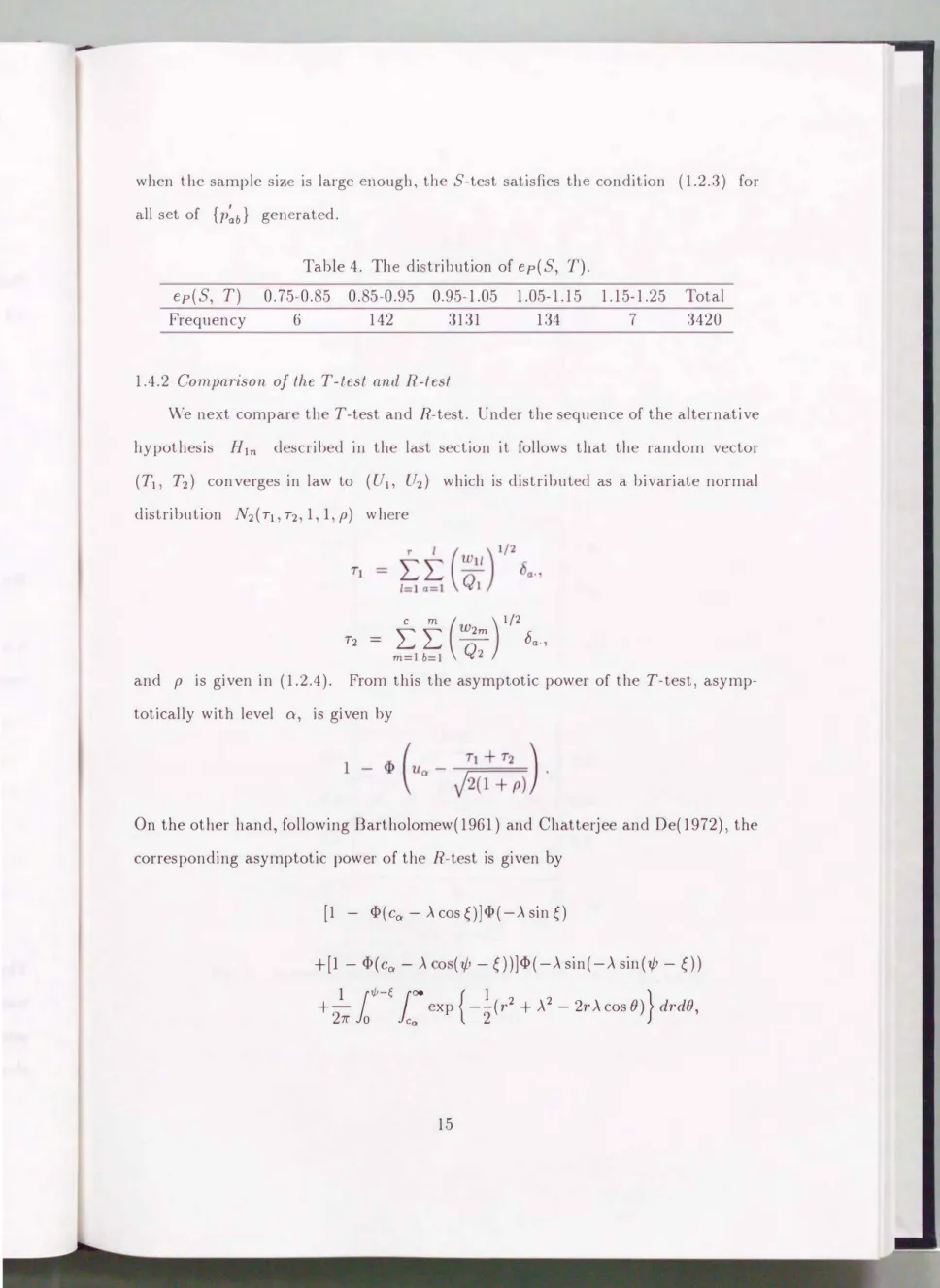
1 4

when the sample siz is large nough, th S-test satisfies th condition (1.2.3) for all s t of

{p�b}

gen rated.

Table 4. Th di tribution of ep(S,

T).

ep(S, T) 0.75-0.85 0.85-0.95 0.95-1.05 1.05-1.15 1.15-1.25 Total

Frequency 6 142 3131 134 7 3420

1.4.2

Comparison of the

T

-test and R-test

We next compar th T-test and R-t st. Und r the sequence of the alternative hypothesis H1n described in the last section it follows that the random vector (T1 T2) converges in law to

(U1, U2)

which is distribut d as a bivariate normal distribution N2(T1,T2,1,1,p) wh re

c

m ( )

^1/2

72 ⁼

_{m=l b=I} L L

^W

^Q

²

^m

₂ ^8a.,

and p is given in (1.2.4). From this the asymptotic power of the T-test asymp­

totically with level a, is given by

On the other hand, following Bartholomew(1961) and Chatterjee and De(1972) the corresponding asymptotic pow r of the R-test is given by

[1

- <I>(ca-

Acos�))<I>(-Asin�)

+[1-

<I>(ca-

A o

(7/J-

�)))<I>( -A sin( -A sin('l/J- �)) 1

11/J-e joo {

¹

+- xp -

-

⁽

^r

2 + A2 - 2r A cos

B) drdB, }

27r 0 c0 2

flr(C,)

0.6 0.6

0.4 0.4

0.2 0.2

0 n n

({,)

6 J

(i) p=-0.5

fJ

1

( {,)

0.6 0.6

0.4 0.4

0.2 0.2

0 n n

((,)

4 2

( ii) p=O.O

fJ

r

( (,)

0.6 0.6

0.4 0.4

0.2 0.2

0 n 2n

(C,)

J J

(iii) p=O.S

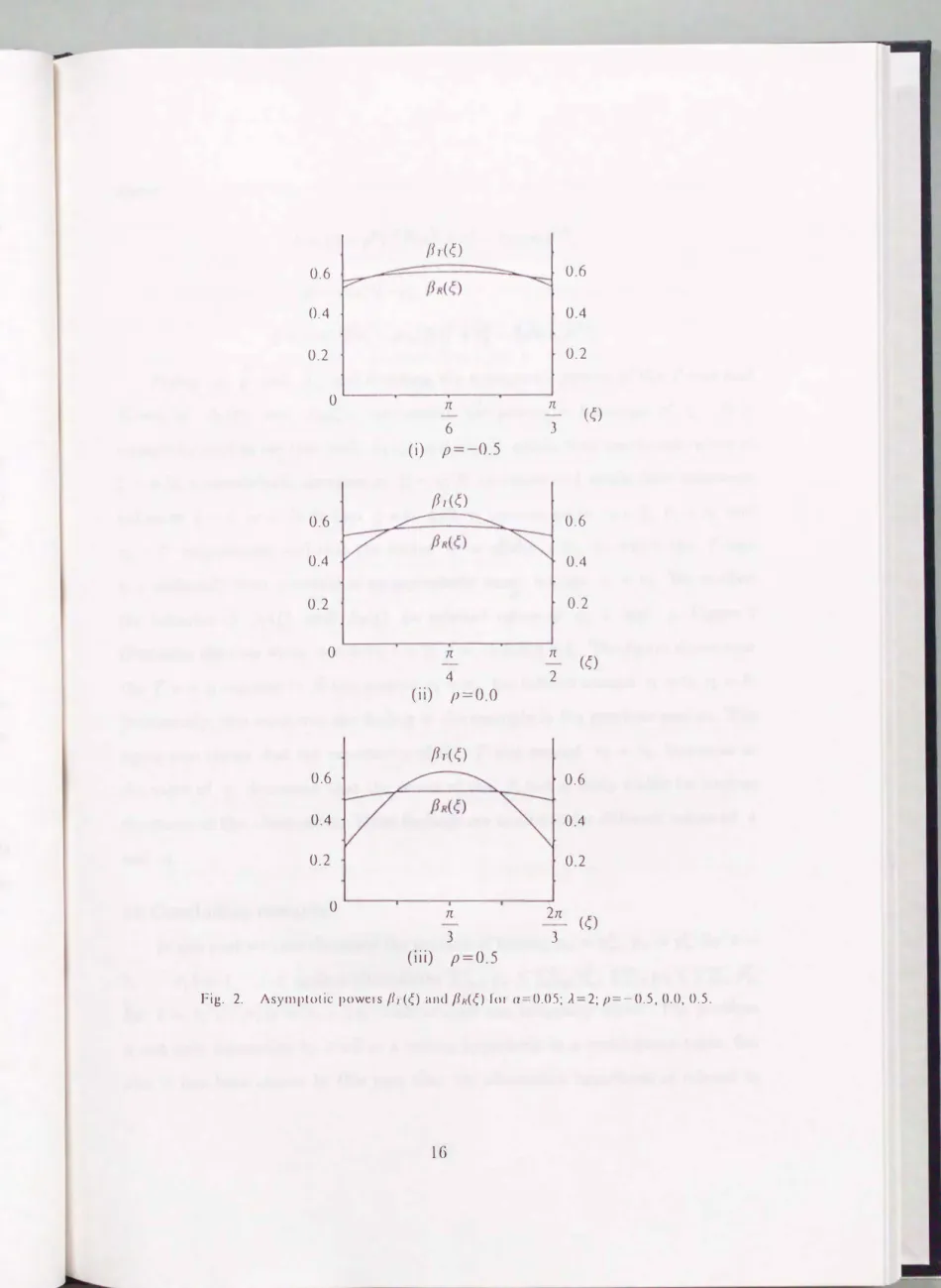
Fig. 2. Asymptotic powers /11 (¢) und flu(¢) for a=0.05; A=2; p=-0.5, 0.0, 0.5.

16

wher

7/J

^{= cos-1(}

-p),

�

⁼ cos-

1[(71- p72)/(712

+

7i- 2p7172)112].

Fixing ^a

p

and .A, and d noting th a ymptotic pow rs of the T-test and R-test by

f3r(�)

and

f3R(�)

w consid r th powers a functions of

�·

It is traightforward to s ^e that both

f3r(�)

and

f3R(�)

attain th ir maximum values at

�

⁼

7/J/2

symmetrically deer as as

I�- 7/J/21

increase and attain their minimum values at � ⁼ 0 or

7/J.

Not that

�

⁼ 0,

7/J/2,

'ljJ corr pond to

72

⁼ 0,

71

⁼

72

and

71

⁼ 0 respectively and that th v ctor

81

⁼

c�d(c

^> 0) to which the T-test is a uniformly most pow rful in an a ymptotic n ^e impli s

71

⁼

72.

We studied the behavior of

f3r(�)

and

f3R(�)

for s lect d valu of ^a .A and p. Figure

2

illustrates the case wh n ^a= 0.05; .A ⁼

2; p

⁼ -0.5, 0.0 0.5. The figure shows that the T-test is superior to R-test around

71

⁼

72

but inf rior around

71

⁼ 0,

72

⁼ 0.

Incidentally this reinforce th finding in th xample in th pr vious section. The figure also shows that the superiority of th T-test around

71

⁼

72

Increase as the value of p decreas s; that the pow r of th R-test is fairly stable for various directions of the alternatives. These findings ar unalter d for different values of .A and ^a.

1.5 Concluding remarks

In this part we hav discuss d th probl m of testing

Pa·

⁼

P�., P-b

⁼

p?b

for ^{a =} 1, ... , r; b ⁼ 1, ...

, c

against alt rnativ

2::::�=1 Pa· :::; 2::::�=1 P�., 2::::�1 P·b :::; I:�1 p?b,

for l ⁼ 1, ... , r, ^{m =} 1, .^{. .}

, c,

with at 1 a t on in quality stri t. Th probl ^rn is not only interesting by its lf as a t ting hypoth sis in a contingency tabl , but also it has been shown in this part that th alt rnativ hypoth is is relat d to

the on -sid d alt rnative in a comparati v study under a bivariate non parametric formulation.

We have consid r d th thr tests, S-te t, T-t st and R-test. The S-test 1s an approximat ly most string nt som wher most pow rful test. The T-test and R-t t combine approximately most stringent som wh re most powerful tests obtained from each marginal of the canting ncy table. Wher as the T-test simply adds, R-test employs the likelihood ratio crit rion for the combination.

The alternative hypoth si is compo it with restriction and it is difficult to compare th three tests in general. W hav consider d the r stricted family of alternativ hypothesi which is g n rat s by a bivariat normal di tribution for the comparison of the S-test and T-test. Al o w hav directly compar d the asymptotic powers of the T-test and R-t st. Under thes s tups it has been shown that the three tests are competitiv r garding th ir a ymptotic power in particular

i

)

T-test is highly comp titiv with th -t t.

ii

)

T-test is superior to th R-test around E

(

^TI

)

^{= E}

(

^T2

)

, but inferior to the R-test around E

[

^T1

]

^{= 0 or E}

[

^T2

]

^{= 0.}

iii

)

The superiority of th T-test around E

[

^T1

]

^E

[

^T2

]

Increase as the correlation of T1 and T2 decreases.

iv

)

The power of th R-test is fairly tabl for various directions of the alter­

natives.

We could not compare the powers of th S-t st and T-t t dir ctly b cause of the involvement of too many paramet r .

The us fulness of th tests has b en shown by the practical data from a case­

control study. It has be n shown that th T-t st has small r p-values than th R-test in the region around th straight lin , T1 = T2.

18

Part

2

APPROXIMATELY SOMEWHERE MOST POWERFUL TESTS FOR MARGINAL HOMOGENEI T Y OF A

SQU ARED TABLE UNDER RESTRICTED

ALTERNATIVES

2.1 Introduction

Paired data measur d on a same seal fr qu ntly arise in many applied statistics.

When variables are classifi d into a number of cat gories, data ar summarized into

a square tabl . For an r x r table, we d not th cell and marginal probabilities by Pij, Pi+ and P+j for i, j ⁼ 1,

. . .

, r, and th corr sponding observations by nij ni+ and n+j for a ample size of n.

For t sting homogen ity of th two marginal distributions;

Ho : Pi+ ⁼ P+i, _i = 1,

.

. . r- 1

Stuart(1955) gave a te t bas d on the tati ti S = d'U-1d where d =

(

n1+-

and Uij = -

(

nij + nji

)

for i # j i j ⁼ 1, .

..

r

-

1. Aft r hi work, Madan­

sky(1963), Bhapker(1966) and Ir land Ku and Kullback(1969) propo ed other tests.

All of these test statistic asymptotically distribute a th chi- quare distribution with r -1 degrees of freedom( H reaft r w abbreviate as

d.f.)

under H0. These test statistics do not incorporate th ordinal prop rty of the variables. In fact, they are invariant to the permutation of the corr ponding rows and columns of the table and so applicable to any nominal cat gorical data. However ordinal data have often a tendency that eith r marginal distribution is stochastically larger than the other.

In practice, such a situation occurs wh n the marginal distributions of the underly­

ing distribution differ only in their location . Here our alternatives are represented as follows:

k k

Hl:

L

Pi+ �

L

P+i,

i=l i=l

k=l, ... ,r-1

or (2.1.1)

k k

L

Pi+ �

L

P+i,

i=l i=l

k=1, ... ,r-1

20

where at least on in quality is strict. For om sp cifi probability models, above hypoth s are d rived naturally. An xa1npl is giv n by the conditional symmetry model·

Pii

⁼

TJ</Jii

(

i

^<

j)

<Pii

⁽

i

⁼

j)' (2-TJ)<Pji (i>j),

where

L:�=l <Pii

+

2 L:i<j <Pij

⁼ 1. On thi mod 1, t sting H0 against H1 reduces to t sting TJ ⁼ 1 again t TJ =f 1. Some models giving ri to th s situations are listed in Agre ti(19

4).

For this testing probl m Agr ti(19

3)

propo ed the Mann-Whitn y test. From

a simulation tudy under an as umption of the bivariate normal distribution with a positive correlation co ffici nt h in i ted on th pow r uperiority of the Mann- Whitney te t over th Bhapkar' test which i ba ed on a chi- quared statistic that uses an estirnat of th non-null covariance matrix in t ad of U in the Stuart's test statistic S. He also recommended t sts ba ed on weighted urns of the marginal differences, but he did not discu in d pth th way how to 1 ct the weights.

In this part these tests based on th weight d urn of marginal differences are called approximately sorn wher most pow rful unbia d(SMPU) te ts as explained in section

2.2.

We must remark that, for orne alternatives in H1, the approximately

SMPU tests may have 1 ss powers than th chi-squar d tests. As a chi-squared test we consider the Stuart's test in thi part. In s ction

2.2

th Mann-Whitney statistic TMw in normalized form is shown to be an approxirnat ly SMPU test statistic. Mor over, an optimal t t among th approximat ly SMPU te t is derived under the most string nt principl . In ction

2.3,

th asymptotic powers of the approximately SMPU t sts and th Stuart' test ar studi d und r the s quenc of alternatives converging to H0. S tion

2.4

i d vot d to xplore th optimal test when a continuous bivariat distribution is assum d a an und rlying di tribution. In section

2.5,

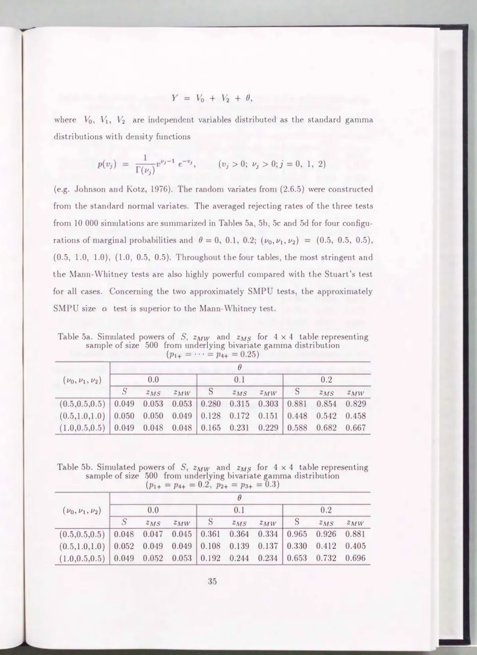
thre tests ar appli d for the unaid d di tan vi ion data. Simulation

study is performed in section 2.6, assuming a bivariate normal distribution and a bivariate gamma distribution a an und dying distribution.

2.2 Approxin1.ately son1ewhere n1ost powerful unbiased tests We denote the cumulative marginal probabilities by

k P[k]+ LPi+,

i=l k' P+[k'] ⁼ LP+j,

j=l

and the corre ponding cumulative observation by n[k]+ and n+[k'J for k, k' 1, ... , r - 1. Then the alternativ s H1 in (2.1.1) is rewritten as

H1 : P[iJ+ < P+[i], ^{z =} 1 ... r- 1, or

P[i]+ � ^{P+(iJ, i =} 1, ... ,r-1,

where at least one inequality is strict. It is easily s en that the vector

has the mean,

nO ⁼ n(P[IJ+ -P+[l], ... , P[r-IJ+ - P+(r-1])'

and the covariance matrix, nE ⁼ n(a-ij), wher

i r

O"ij ⁼ L L (Pst + Pts) -(P(i]+ -P+(i]) (P[j]+ -P+[j]) s=lt=j+l

for 1 S i S j S r - 1. Especially, und r H0, we have (J ⁼ o and

t r

O"ij ⁼ L L (Pst + Pts) s=lt=j+l

22

with p's sati fying H0. Throughout this part w assume the covariance matrix � to be nonsingular. For testing 1-!0 again t

H1,

the statistics in our considerations are all repre en ted in t rm of c. In fact, th Stuart's test statistic can be rewritten as S ⁼ c'V

- 1

^{c, wh r} V

= ( Vij)

^with

Vij = L::=1 L:;=j+1 ( nst

+

nts)

^for

1 :s; i :s;

j :s; r-

^1. For testing H0 against H1, Agresti

(

¹⁹

3)

recommend d the use of the Mann-Whitney statistic,

TMw ⁼

l:::(ni+n+j- nj+n+i)·

i<j

Note that TMw

/n

detects the probability cliff r nee,

P(X

^<

Y) - P(X

^>

Y),

provided that

X

^and

Y

are ind p nd ntly di tributed as the multinomial distri­

butions

P(X

⁼

i) =Pi+,

^and

P(Y = j) = P+j

^for

i j = 1 ... , r

respectively. As is well-known the Mann-Whitn y stati tic TMw alg braically coincides with the Wilcoxon statistic

Moreover we can easily show that

r-1

TMw

= l:::(ni+

+

n(i+1)+)(n[i]+- n+[iJ) i=1

= - L(n+i r-1

+

n+(i+1))(n+[i] - n[i]+)·

i=1

Thus we have

Proposition 1.

The Mann- Whitney tatistic is expr ed as

1

r-1

TMw

= ₂ � ⁽ⁿⁱ⁺

⁺

ⁿ⁺ⁱ

⁺

^n(i+1)+

⁺

n+(i+1))(n[i]+- n+[iJ)·

l=1

Agresti also suggest d the tests based on w ight d urns of marginal cliff r n s,

r-1

Tw = L w;(ni+- n+i),

i=1

but he did not discuss nough th s 1 ction of th w ights. To r present the statistic according to the alt rnative hypoth ses, w employ

r-1

Tw ₌

L Wi(n[i]+- n+[ij).

i=1

From the larg sampl th ory, the statistic

yin( n -1 c - 8)

asymptotically distributes as

Nr_1 ( o, �)

that is, the

(

^r

- 1

)-variate normal distribution with mean

o

and covariance matrix

�.

Let

X

=

(X1, ... , Xr_t)'

be distributed as

Nr_1(v, f)

with known r. We also us the notation

v::; (�)o

which means that all component of

v

are nonpositive (nonn gativ

)

. For testing the null hypothesis,

v

=

o,

against th alternatives,

v ::; o

or

v � o ( v =f o)

consider a test given by;

Reject the null hypothesi if

lw' X II vw'fw

_�

Uaj2

wh re

w � o(

^w

=f

⁰

)

and

ua;2

is the upper

a/2

quantile of the tandard normal distribution. This test is the most powerful unbiased size

a

t st again t the alternative

{v· v

= kr

-1

^{w k}

=f 0}

and therefore it is called a som wh r most powerful unbia ed(SMPU) size

a

test (Schaafsma and Smid,

1966).

In our probl m of testing

H0

against

H1,

we call the approximated test based on

w'cjvw'Vw

an approximately SMPU test. We remark that the weight vector

w

may d pend on the ample. In fact, the normalized Mann- W hitney test stati tic is given by

zMw =

1r'cjV1r'V1r

with

1r

⁼

n-1(n1+

⁺

n+1

⁺

n2+

⁺

n+2, ... , n(r-1)+

⁺

n+(r-1)

⁺

nr+

⁺

n+rY·

We consider an optimal test among th approximat ly SMPU te ts employing the most stringent principle explored by Schaafsma and Smid

(1966).

Let C _b the class of SMPU size

a

tests for

v

=

o

against

v ::; o

or

v � o( v =f o)

and

f3ct>( v)

be the power of th test ¢ E C _at

v.

Mor over w u th notation

lct>,c(v)

=sup

(31/l(v)- f3ct>(v),

1/;EC

24

which is called the shortcorning of the t st

¢

^{among C.} The most stringent SMPU size a test is d fin d by th SMPU iz a test

¢

that satisfies

supf'¢,c(v) = inf sup/,p,c(v).

v�O ^1/;EC v�O

Thu the most tring nt SMPU t st is th SMPU t t that minimiz s the maximum shortcoming arnong th SMPU t sts( For d tails Schaafsma and Smid, 1966

)

^{. We}

apply this test approximately in our situation, and w call th test an approximately most string nt SMPU size a test.

Put v-1 = (

vij)

^and

e

₌

_{fo( #,}

· · ·

Jvr-1,r-1

⁾

'

_. Then, from Theorem 2.1 of part 1 with a minor modification for th two-sided alternativ s we have

Proposition 2. The approximat ly mo t tringent SMP U te t is given by the statistic

ZMW =

e'c!/e've.

2.3 Comparison of the asymptotic powers

To see the behavior of these test stati tics in a neighborhood of p's satisfying

H0,

we consider the following s qu nee of alternatives according to the sample size

where

Pi+

⁼

P+i,

^{i = 1,} . . . , r and

8'

satisfy (i)

I::i=1 2::j=1 8ij

^{= 0; (ii)}

8[i)+

⁼

I::i=18k+

= 0 fori= 1, .

.

^{. ,r -1; (iii)}

8+[i)

⁼

I:i=18+k:::;

^{0 for i = 1,}

..

^{. ,r -1 or}

8+[i)

^{� 0 for i=} 1, ... ,r- 1, withat l a t on in quality b ing stri t. Unci r

H1(n),

as n tends to infinity, the Stuart's stati tic S conv rges in law to the none ntral chi-square distribution,

x;_1(1'�-11)

(cf. Bishop, Fi nb rg and Holland, 1975

)

^with

r -1 d. f. and noncentrality par am t r

1'�-11

^{wh r}

1

^{= (}

8+[1] ... , 8+[r-1] ) '

and

�

consists of p's.

Under

Hin),

the statisti ,

Zw ==

w'ciVw'Vw,

with a constant vector

w

⁼⁼

(

^WI, .. . , Wr-

d

^' conv rges in law , as n ---+ oo, to the normal di tribution with m an

-w'IIVw''L.w

and unit variance. Similarly, for

zMw and ZMs, we have

Proposition 3.

The tatistics

ZMW

and

ZM

asymptotically distribute as the

normal di tributions with unit variances and m an , - 1r _�

1

1 .j1r�r.1ro, -e.�, ₁ .J e�r.eo)

respectively, where 1ro

==

(PI+

⁺

P+I

⁺

P2+

⁺

P+2 ... , P(r-I)+

⁺

P+{r-I)

⁺

Pr+

⁺

P+r )'

and f..0

⁼⁼

( y'ail,

^.

^.

^.

, J O"r-I,r-I )'

^,

^provided ( O"ij)

⁼⁼

r_-I.

The asymptotic pow r function of the t st ba ed on Zw is given by

where <I>( x) is the standard normal di tribution function. W r trict 8's so a

/'r.-I/

⁼⁼

^A

for a fixed

A.

Thus th t st ba d on Zw is an asymptotically most powerful unbiased size a test again t th alt rnativ where 1 ==

kr.w

for a constant

k,

when the power is given by

Let

X�,I-a

be the upper a-quanti! of th 2-distribution with

k ^d.f.,

^{and put}

We also define

1-la(/3)

by the positiv solution of 11 to th equation,

Then we have

Proposition 4.

For a positive constant

TJ,

th test bas d on

Zw

has the power larger than or equal to

TJ ^•

/3r-I

^(a,

A) if and only if

26

jw'rl/v'w'�w

_2:

lla(17

^·

f3(a, A)). (2.3.3)

Let ^T be the angl between the vectors

1

and

�w

with r spect to the inner product,

(a, b)= a'�-1b.

Then the inequality

(2.3.3)

is equivalent to

>

lla(7]·/3r-1(a,A))

COST

1\ .

- VA

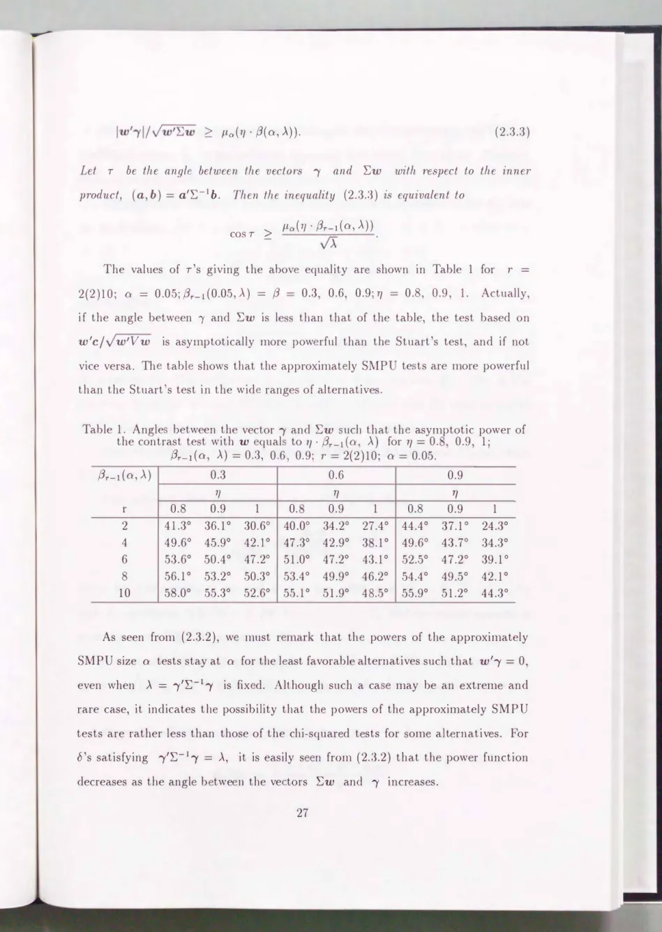
The values of ^T 's giving the abov equality ar shown in Table

1

for r

= 2(2)10; a = 0.05; f3r-I (0.05, A) = /3 0.3 0.6 0.9;

7]

= 0.8, 0.9, 1.

Actually, if the angle betw en 1 and

�w

is 1 than that of the table, the test based on

w' cj J w'V w

is asytnptotically more pow rful than th Stuart's test, and if not

vice versa. Th tabl shows that the approximat ly SMP te ts are more powerful than the Stuart's test in the wid rang s of alternativ .

Table

1.

Angle betw en th vector

1

and

�w

uch that th asymptotic power of the contrast te t with

w

qual to

17

^·

f3r-I (a A)

for 77 ⁼

0. 0.9 1·

f3r-l(a, A)= 0.3, 0.6 0.9;

r

= 2(2)10; a= 0.05.

f3r-l(a, A) 0.3 0.6 0.9

7]

_{7] 7]}

r

0.8 0.9 1 0. 0.9 1 0.8 0.9 1

2 41.3° 36.1° 30.6° 40.0° 34.2° 27.4° 44.4° 37.1° 24.3°

4 49.6° 45.9° 42.1° 47.3° 42.9° 3 .1 ° 49.6° 43.7° 34.3°

6 53.6° 50.4° 47.2° 51.0° 47.2° 43.1° 52.5° 47.2° 39.1°

8 56.1° 53.2° 50.3° 53.4° 49.9° 46.2° 54.4° 49.5° 42.1°

10 58.0° 55.3° 52.6° 55.1° 51.9° 4 .5° 55.9° 51.2° 44.3°

As seen from

(2.3.2),

w must r mark that th pow rs of the approximately SMPU size

a

tests stay at

a

for the 1 ast favorabl alternatives such that

w'r = 0

even when

A = 1'�-Ii'

is fix d. Although such a ca may be an xtrem and rare case, it indicates th possibility that th pow rs of th approximately SMPU tests are rather less than those of the chi-squar d t sts for om alt rnativ s. For 8's satisfying

r'�-li' = A,

it is easily s ⁿ from

(2.3.2)

that th pow r function decreases as the angl b twe ⁿ the ve tors

�w

and

1

incr as s.

Concerning the approximat ly mo t stringent SMPU test statistic, the limiting coefficient v ctor

eo

is g nerally not xpr ss d in a simpl form of p's. However, some cases giv relativ ly sitnpl xpr sswns.

Propo ition 5. Wh

n the va1·iabl s in each pair are independent under H0, that zs, Pii

=

Pi+P+i for i, j

= 1, ..

. , r, we have

� ( -1-+

¹

)

2

Pi+ P(i+t)+ ' and therefore

for a constant

k.

Esp cially when PI+

⁼

P2+

⁼

. .

^{. =}

Pr+' we have eo

⁼

k'1ro

^{= k"1}

for some constants k' ^and k", ^with

^{1 =}

(1

^{... 1}

^)' and thu the most stringent

SMPU

test a ymptotically coincid with the Mann- Whitney t st.

From the definition of the mo t string nt SMP t st(Schaafsma and Smid,1966), it follows:

Proposition 6.

For

8'

sati fying

A ⁼

1'2:-11, we have

where the first equality is attain d at 1

= kiei,

with ei

⁼

(0, ... , 0 (1), 0, ... , 0)

and

ki

satisfying r'2:-1r

^{= A}

^{for i}

^{= 1,}

. .. , r -

1,

and the second equality is given by 1

=

k'2:e0 for a con tant k'.

Thus the possible minimum pow ^r of th most stringent SMPU test d pends only on X =

.j ^e�2:eo

for fix d A and so X is an ind ^X for th po ibl minimum power.

Proposition 7.

When O"ij Py'CJiiO"jj for i =/= j, we hav (r

-1){1

+ ^(r-

^3)p}

1-p 28